Logarithmic sized proofs of commitment

In a previous chapter, we showed that multiplying the sums of elements of the vectors $\mathbf{a}$ and $\mathbf{G}$ computes the sum of the outer product terms, i.e. $\sum \mathbf{a}\otimes\mathbf{G}=\sum\mathbf{a}\sum\mathbf{G}$. We also showed that the outer product “contains” the inner product along its main diagonal.

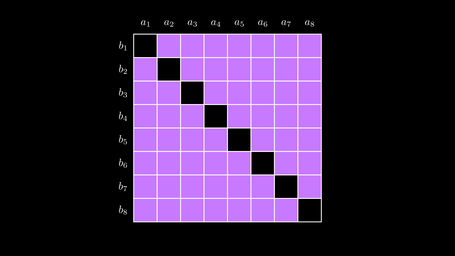
To “extract” the inner product $\langle\mathbf{a},\mathbf{G}\rangle$, one must subtract from the outer product all terms that are not part of the inner product, i.e. the purple shaded region below:

There are $\mathcal{O}(n^2)$ such terms, so doing this directly is not efficient.

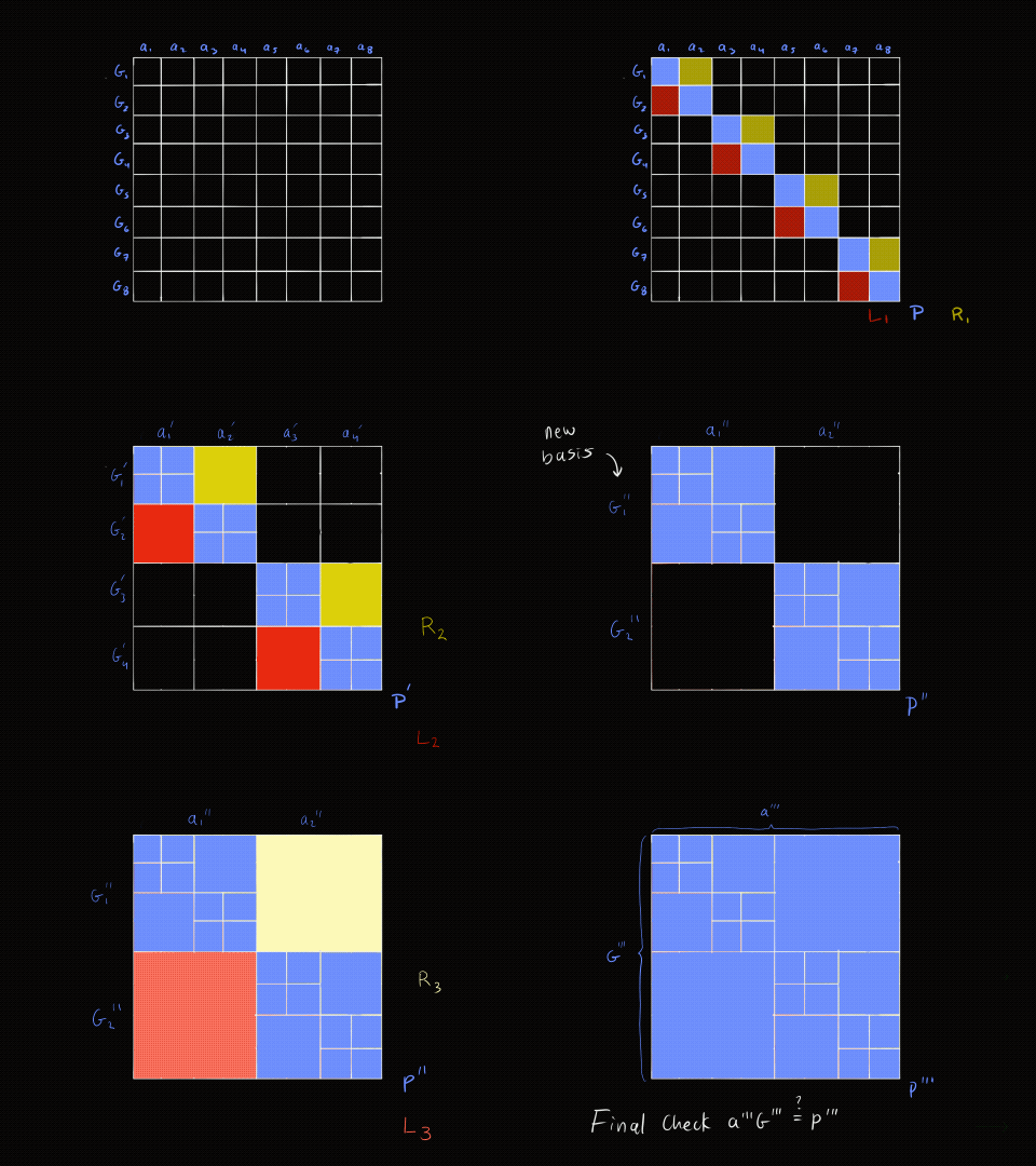
However, observe that we can “fill up the outer product” in the manner shown in the animation below:

In the animation above, after the prover sends the off-diagonal terms, the prover folds both $\mathbf{G}$ and $\mathbf{a}$, reducing their length by half.

At the end, after we have folded $\mathbf{a}$ and $\mathbf{G}$ $\log n$ times, the size of the vectors is 1. When $n=1$ the outer product equals the inner product and we simply reveal both vectors, which will be of constant size.

Recap — and how this relates to the previous chapter’s algorithm

Previously, we showed how to prove we know the opening to a commitment $P$ while sending $n/2$ elements instead of $n$. As a recap:

The prover commits the vector $\mathbf{a}$ to $P$ as $P = \langle\mathbf{a},\mathbf{G}\rangle$. The prover then sends the off-diagonal terms $L=a_1G_2 + a_3G_4 + \dots a_{n-1}G_n$ and $R = a_2G_1 + a_4G_3 + \dots a_nG_{n-1}$. The verifier responds with $u$ and the prover folds the vector $\mathbf{a}$ over $u$ as $\mathbf{a}’=\mathsf{fold}(\mathbf{a},u)=[a_1u+a_2u^{-1}, a_3u+a_4u^{-1}, \dots, a_{n-1}u+a_nu^{-1}]$ and sends $\mathbf{a}’$ to the verifier. Since $\mathbf{a}’$ is of length $n/2$, we have cut the size of the data to be transmitted in half.

The verifier then checks that $\langle\mathsf{fold}(\mathbf{G},u^{-1}),\mathbf{a}’\rangle\stackrel{?}=Lu^2+P+Ru^{-2}$

The original intent of this algorithm was to prove that we know the commitment to $P$ by showing that we know the sum of the inner product $P$ and the off-diagonal terms $L$ and $R$ equals the sum of the elements of the outer products of the pairwise partitions of $\mathbf{a}$ and $\mathbf{G}$.

If we recursively apply this algorithm, we get the $\log n$ algorithm described at the beginning of this chapter.

However, we could also interpret this procedure as us proving we know the opening to the commitment $P’$ where $P’=(Lu^2+P+Ru^{-2})$ with respect to the basis vector $\mathsf{fold}(\mathbf{G},u^{-1})$ of length $n’=n/2$. We could naïvely prove we know the opening of $P’$ by sending $\mathbf{a}’$ and the verifier checking that $P’\stackrel{?}=\langle\mathbf{a’},\mathsf{fold}(\mathbf{G},u^{-1})\rangle$.

But rather than proving we know the opening to $P’$ by sending $\mathbf{a}’$, we can recursively apply the algorithm to prove we know the opening to $P’$ by sending a vector $\mathbf{a}{\prime\prime}$ of size $n/4$. In fact, we can keep recursing until $a^{\prime\dots\prime}$ is of size $n=1$.

The animation below provides an intuition of what is happening. The next section describes the animation in detail.

For this algorithm to work, the length of the vectors must be a power of two. However, if the length is not a power of two, we can pad the vectors with zeros until the length is a power of two.

Proving we know the opening to $P$ with $\mathcal{O}(\log n)$ data

The algorithm

The prover and verifier agree on a basis vector $\mathbf{G}$ of length $n$. The prover sends the verifier $P$ which is $\langle\mathbf{a},\mathbf{G}\rangle$. The prover wishes to convince the verifier that they know the opening to $P$ while sending only logarithmic-sized data.

The prover and verifier then engage in the following algorithm below. The arguments after the | mean they are only known to the prover.

In the algorithm description below $n$ is the length of the vectors in the input, which are all of the same length.

$\texttt{prove_commitments_log}(P, \mathbf{G}, | \mathbf{a})$

Case 1: $n = 1$

1. The prover sends $a$ and the verifier checks that $aG \stackrel{?}= P$ and the algorithm ends.

Case 2: $n > 1$

1. The prover computes and sends to the verifier $(L, R)$ where $$\begin{align*} L &= a_1G_2 + a_3G_4 + \dots a_{n-1}G_n\\ R &= a_2G_1 + a_4G_3 + \dots a_nG_{n-1} \end{align*} $$
2. The verifier sends randomness $u$
3. The prover and verifier both compute: $$ \begin{align*} \mathbf{G}’&=\mathsf{fold}(\mathbf{G},u^{-1})\\ P’ &= Lu^2+P+Ru^{-2} \end{align*} $$
4. The prover computes $$\mathbf{a}’=\mathsf{fold}(\mathbf{a},u)$$
5. $\texttt{prove_commitments_log}(P’, \mathbf{G}’, \mathbf{a}’)$

Commentary on the algorithm

The prover is recursively proving that, given values $P$ and $\mathbf{G}$, they know the $\mathbf{a}$ such that $P=\langle\mathbf{a},\mathbf{G}\rangle$. Both parties recursively fold $\mathbf{G}$ until it is a single point, and the prover recursively folds $\mathbf{a}$ until it is a single point.

The prover transmits a constant amount of data on each iteration, and the recursion will run at most $\log n$ times, so the prover sends $\mathcal{O}(\log n)$ data.

We stress that this algorithm is not zero knowledge because in the case $n=1$, the verifier learns the entire vector. The verifier could also send non-random values for $u$ to try to learn something about $\mathbf{a}$.

However, recall that our motivation for this algorithm is to reduce the size of the check $t_u=\langle\mathbf{l}_u,\mathbf{r}_u\rangle$, and $\mathbf{l}_u$ and $\mathbf{r}_u$ were not secret to begin with.

In fact, we have not shown how to prove we know the inner product with logarithmic-sized data, we have only shown that we know the opening to a commitment with a logarithmic-sized data. However, it is straightforward to update our algorithm to show we know the inner product of two vectors, as we will do later in this article.

Runtime

The verifier carries out the computation $\mathbf{G}’ = \mathsf{fold}(\mathbf{G}, u^{-1})$ $\log n$ times, and the first $\mathsf{fold}$ takes $\mathcal{O}(n)$ time. At first glance, it seems that the verifier’s runtime is $\mathcal{O}(n \log n)$. However, notice that with each iteration, $n$ is halved, resulting in a runtime or $n + \frac{n}{2} + \frac{n}{4} + … + 1 = 2n$, leading to an overall runtime for the verifier of $\mathcal{O}(n)$.

Proving we know the inner product $\langle\mathbf{a},\mathbf{b}\rangle=v$

We now adjust the algorithm above to prove that we conducted the inner product between two scalar vectors, as opposed to a vector of field elements and a vector of elliptic curve points.

Specifically, we must prove that $P$ holds a commitment to the inner product $\langle\mathbf{a},\mathbf{b}\rangle$. This inner product is a scalar, so we do a normal Pedersen commitment instead of a vector commitment. For this we use a random elliptic curve point (with unknown discrete log) $Q$. Thus, $P = \langle\mathbf{a},\mathbf{b}\rangle Q$.

However, we cannot simply re-use our previous algorithm because the prover can provide multiple openings to $P$. For example, if $\mathbf{a} = [1,2]$ and $\mathbf{b} = [3,4]$, the prover can open also open with vectors $\mathbf{a}’ = [3,2]$ and $\mathbf{b}’ = [1, 4]$.

To create a secure proof of knowledge of an inner product, the prover must also compute and send a commitment for $\mathbf{a}$ and $\mathbf{b}$.

The naive solution is to run the commitment algorithm twice. The first two times are to prove $\mathbf{a}$ and $\mathbf{b}$ are properly committed to $P_1 = \langle\mathbf{a},\mathbf{G}\rangle$ and $P_2 =\langle\mathbf{b},\mathbf{H}\rangle$ and the third time is to show that $\langle\mathbf{a},\mathbf{b}\rangle Q=P_3$ was properly computed. In the next section, we show how to modify our algorithm to compute the inner product when both vectors are field elements.

Converting a scalar inner product to a scalar-point inner product

Let $\mathbf{Q}^n$ be the vector consisting of $n$ copies of the point $Q$, i.e.

$$\mathbf{Q}^n=[\underbrace{Q,\dots, Q}_n]$$

Thus,

$$\mathbf{b}\circ\mathbf{Q}^n=[b_1Q, b_2Q,\dots,b_nQ]$$

Note that $\langle\mathbf{a},\mathbf{b}\rangle Q$ is equal to $\langle\mathbf{a},\mathbf{b}\circ\mathbf{Q}^n\rangle$.

That is, we can multiply each entry of $\mathbf{b}$ by $Q$ and take the inner product of that vector with $\mathbf{a}$ and the result will be the same as $\langle\mathbf{a},\mathbf{b}\rangle Q$. For example, if $\mathbf{a} = [1,2]$ and $\mathbf{b} = [3,4]$, then $\langle[1,2],[3,4]\rangle Q=(1\cdot 3+2\cdot 4)Q= \langle[1,2],[3Q,4Q]\rangle=1\cdot 3Q+2\cdot 4Q=11Q$.

From there, we could prove the following:

1. $P_1 =\langle\mathbf{a},\mathbf{G}\rangle$
2. $P_2 =\langle\mathbf{b},\mathbf{H}\rangle$
3. $P_3 =\langle\mathbf{a},\mathbf{b}\circ\mathbf{Q}\rangle$

One proof instead of three

We can do better than sending three commitments and run the algorithm three times.

Because the points in $\mathbf{G}$, $\mathbf{H}$ and $Q$ have an unknown discrete log relationship, they can be combined as a single commitment $P = \langle\mathbf{a},\mathbf{G}\rangle +\langle\mathbf{b},\mathbf{H}\rangle + \langle\mathbf{a},\mathbf{b}\rangle Q = P_1 + P_2 + P_3$.

We will slightly re-arrange the commitment $P = \langle\mathbf{a},\mathbf{G}\rangle +\langle\mathbf{b},\mathbf{H}\rangle + \langle\mathbf{a},\mathbf{b}\rangle Q$ as $P = \langle\mathbf{a},\mathbf{G}\rangle+\langle\mathbf{a},\mathbf{b}\circ\mathbf{Q}^n\rangle +\langle\mathbf{b},\mathbf{H}\rangle$ to make the next trick more obvious.

To prove this entire commitment at once, instead of three inner products, observe that

$$P=\langle\mathbf{a},\mathbf{G}\rangle+\langle\mathbf{a},\mathbf{b}\circ\mathbf{Q}^n\rangle +\langle\mathbf{b},\mathbf{H}\rangle=\langle\mathbf{a}\oplus\mathbf{a}\oplus\mathbf{b},\mathbf{G}\oplus\mathbf{Q}^n\oplus\mathbf{H}\rangle$$

where $\oplus$ means vector concatenation.

Effectively, we are proving we committed vector $\mathbf{a}\oplus\mathbf{a}\oplus\mathbf{b}$ to elliptic curve vector basis $\mathbf{G}\oplus\mathbf{Q}^n\oplus\mathbf{H}$.

In practice, we don’t actually concatenate the vectors because the total length would generally not be a power of two. Rather, we compute the $\mathbf{G}$, $\mathbf{H}$, and $\mathbf{b}\circ\mathbf{Q}^n$ components separately, but compute $L$ and $R$ as if they were concatenated.

We show the algorithm in the animation below:

The algorithm

Given $v = \langle\mathbf{a},\mathbf{b}\rangle$ and commitment $P = vQ+\langle\mathbf{a},\mathbf{G}\rangle + \langle\mathbf{b},\mathbf{H}\rangle$ we wish to prove that $P$ is committed as claimed. That is, $v$, $\mathbf{a}$, and $\mathbf{b}$ are committed to $P$ and $\langle\mathbf{a},\mathbf{b}\rangle=v$.

$\texttt{prove_commitments_log}(P, \mathbf{G}, \mathbf{H},Q, |\mathbf{a}, \mathbf{b})$

Case 1: $n = 1$

1. The prover sends $(a,b)$ and the verifier checks that $P \stackrel{?}= aG + bH + abQ$. The algorithm ends.

Case 2: $n > 1$

1. The prover computes and sends to the verifier $(L, R)$ which are simply the off-diagonal terms of all the vectors concatenated together (see the animation above): $$\begin{align*} L &= (a_1b_2 + a_3b_4 + \dots a_{n-1}b_n)Q+(a_1G_2 + a_3G_4 + \dots a_{n-1}G_n)+(b_2H_1 + b_4H_3 + \dots b_nH_{n-1})\\ R &= (a_2b_1 + a_4b_3 + \dots a_nb_{n-1})Q+(a_2G_1 + a_4G_3 + \dots a_nG_{n-1})+(b_1H_2 + b_3H_4 + \dots b_{n-1}H_n) \end{align*} $$
2. The verifier sends randomness $u$.
3. The prover and verifier both compute: $$ \begin{align*} P’ &= Lu^2+P+Ru^{-2}\\ \mathbf{G}’&=\mathsf{fold}(\mathbf{G}, u^{-1})\\ \mathbf{H}’&=\mathsf{fold}(\mathbf{H}, u)\\\\ \end{align*} $$
4. The prover computes: $$ \begin{align*} \mathbf{a}’&=\mathsf{fold}(\mathbf{a},u)\\ \mathbf{b}’&=\mathsf{fold}(\mathbf{b},u^{-1}) \end{align*} $$
5. $\texttt{prove_commitments_log}(P’, G’, H’, \mathbf{a}’, \mathbf{b}’)$

The following exercises can be found in our ZK Bulletproofs GitHub Repo:

Exercise 1: Fill in the missing code below to implement the algorithm to prove that $\mathbf{a}$ is committed to $\mathbf{G}$ to produce point $P$:

from py_ecc.bn128 import G1, multiply, add, FQ, eq, Z1
from py_ecc.bn128 import curve_order as p
import numpy as np
from functools import reduce
import random

def random_element():
    return random.randint(0, p)

def add_points(*points):
    return reduce(add, points, Z1)

# if points = G1, G2, G3, G4 and scalars = a,b,c,d vector_commit returns
# aG1 + bG2 + cG3 + dG4
def vector_commit(points, scalars):
    return reduce(add, [multiply(P, i) for P, i in zip(points, scalars)], Z1)

# these EC points have unknown discrete logs:
G_vec = [(FQ(6286155310766333871795042970372566906087502116590250812133967451320632869759), FQ(2167390362195738854837661032213065766665495464946848931705307210578191331138)),
     (FQ(6981010364086016896956769942642952706715308592529989685498391604818592148727), FQ(8391728260743032188974275148610213338920590040698592463908691408719331517047)),
     (FQ(15884001095869889564203381122824453959747209506336645297496580404216889561240), FQ(14397810633193722880623034635043699457129665948506123809325193598213289127838)),
     (FQ(6756792584920245352684519836070422133746350830019496743562729072905353421352), FQ(3439606165356845334365677247963536173939840949797525638557303009070611741415))]

# return a folded vector of length n/2 for scalars
def fold(scalar_vec, u):
    pass

# return a folded vector of length n/2 for points
def fold_points(point_vec, u):
    pass

# return (L, R)
def compute_secondary_diagonal(G_vec, a):
    pass

a = [4,2,42,420]

P = vector_commit(G_vec, a)

L1, R1 = compute_secondary_diagonal(G_vec, a)
u1 = random_element()
aprime = fold(a, u1)
Gprime = fold_points(G_vec, pow(u1, -1, p))

L2, R2 = compute_secondary_diagonal(Gprime, aprime)
u2 = random_element()
aprimeprime = fold(aprime, u2)
Gprimeprime = fold_points(Gprime, pow(u2, -1, p))

assert len(Gprimeprime) == 1 and len(aprimeprime) == 1, "final vector must be len 1"
assert eq(vector_commit(Gprimeprime, aprimeprime), add_points(multiply(L2, pow(u2, 2, p)), multiply(L1, pow(u1, 2, p)), P, multiply(R1, pow(u1, -2, p)), multiply(R2, pow(u2, -2, p)))), "invalid proof"

Exercise 2: Modify the code above to implement the algorithm that proves $P$ holds a commitment to $\mathbf{a}$, $\mathbf{b}$ and $v$, and that $\langle\mathbf{a},\mathbf{b}\rangle=v$. Use the following basis vector for $\mathbf{H}$ and EC point $Q$:

H = [(FQ(13728162449721098615672844430261112538072166300311022796820929618959450231493), FQ(12153831869428634344429877091952509453770659237731690203490954547715195222919)),
    (FQ(17471368056527239558513938898018115153923978020864896155502359766132274520000), FQ(4119036649831316606545646423655922855925839689145200049841234351186746829602)),
    (FQ(8730867317615040501447514540731627986093652356953339319572790273814347116534), FQ(14893717982647482203420298569283769907955720318948910457352917488298566832491)),
    (FQ(419294495583131907906527833396935901898733653748716080944177732964425683442), FQ(14467906227467164575975695599962977164932514254303603096093942297417329342836))]

Q = (FQ(11573005146564785208103371178835230411907837176583832948426162169859927052980), FQ(895714868375763218941449355207566659176623507506487912740163487331762446439))

This tutorial is part of a series on Bulletproof ZKP.