Circle FFT — Part 1: Building the Circle Domain

Circle STARKs is a new zk-STARK scheme that has been implemented in Stwo and Plonky3, and it has been adopted by several zkVM projects. Its key innovation lies in enabling the use of small 32-bit fields (Mersenne prime $2^{31}-1$) while still maintaining the mathematical properties needed for efficient FFT operations. In this explanatory article series, we will discuss the primary algorithm behind Circle STARK, named Circle FFT.

In Part 1 article, we first review how STARK-friendly primes have evolved, and then we explore the foundational concepts of Circle FFT—namely the circle curve, its group structure, and the roles of twin-cosets and standard-position cosets, using detailed examples and derivations. Then, in Part 2 article, we will describe the Circle FFT algorithm itself in detail.

We also provide a walkthrough of these core ideas—such as the circle group and the Circle FFT—together with explicit example computations for $p=31$ (Mersenne prime with exponent $5$: $2^5 -1$ ) with Python-script.

Our focus is on how each of these building blocks leads into a full-fledged FFT-like routine even when $p-1$ does not have a large two-adic factor.

If you’re interested in running the examples yourself, the full Python code is available here, and we will reference it in later sections such as Section 4 and 6, where we walk through the group and domain construction in code.

This article was written by Yugo in collaboration with RareSkills. This article was funded by a Soulforge Grant. We are grateful for their support.

0. From STARK‑Friendly Primes to Mersenne 31

Before diving into STARK-friendly prime, let’s first recall finite-field basics.

A field is a set in which addition, subtraction, multiplication, and division (except by zero) are defined. When the set of elements is finite, it is called a finite field. $\mathbb{F}_p$ refers to the set of integers from $0$ up to $p-1$ (where $p$ is a prime), with addition, subtraction, and multiplication all taken modulo $p$, and division defined as the inverse of multiplication modulo $p$.

We denote by $\mathbb{F}_p^*$ the set $\mathbb{F}_p \setminus \{0\}$. Each element in $\mathbb{F}_p^*$ has a multiplicative inverse, so $\mathbb{F}_p^*$ can be viewed as a multiplicative group. The size of this group, $|\mathbb{F}_p^*|$, is $p-1$. When we factorize $p-1$ into its prime factors, it is known that if a prime $q$ appears $r$ times, then there is a cyclic subgroup of size $q^r$.

You can briefly illustrate this with a small prime, for example $p=7$. Since $p-1=6$ factors as $2\times 3$, there must be subgroups of sizes $2$ and $3$. Indeed, in $\mathbb{F}_7^* = \{1,2,3,4,5,6\}$, the element $6$ generates a size-$2$ subgroup $\{1,6\}$, and the element $2$ generates a size-$3$ subgroup $\{1,2,4\}$.

In many STARK protocols, the Number-Theoretic Transform (NTT) or Fast Fourier Transform (FFT) relies on such a subgroup where the factor is a power of 2, so that the subgroup has size $2^r$. The largest integer $r$ such that $2^r$ divides $(p-1)$ is called the two-adicity. A high two-adicity allows a larger power-of-2 size for FFT/NTT domains, which is key to achieving fast polynomial evaluations, interpolations, and polynomial multiplication. Moreover, implementing these NTT-based operations efficiently heavily depends on fast modular multiplications—since FFT/NTT involves repeatedly multiplying elements and reducing them modulo $p$.

Originally, STARKs used a prime $p = 2^{251} + 17 \cdot 2^{192} + 1$, which has a two-adicity of $192$. In modern STARK implementations, one of the improvements was made to reduce overhead by decreasing the size of the finite field. For example, the Goldilocks field is $p = 2^{64} – 2^{32} + 1$ and has a two-adicity of $32$. Crucially, because $2^{64} \equiv 2^{32} – 1 \pmod{p},$ the product of two 64-bit numbers can be split in base $2^{32}$ and reduced with only a few additions and subtractions.

What about Circle STARKs? As proposed in the Circle STARKs paper, it uses a Mersenne prime,

$$ p = 2^{31} – 1.$$

A Mersenne prime is a prime number of the form $2^n -1$ for some integer $n$. Here, $n=31$ gives $2^{31}−1$, which happens to be prime and is therefore categorized as a Mersenne prime.

One primary reason to choose $2^{31}-1$ is that it fits within a 32-bit machine word, making modular multiplication extremely fast. Specifically, when two 32-bit numbers are multiplied, the result is a 64-bit value, and modular reduction by $2^{31}-1$ can be done with only two additions.

This operation can be much faster with vectorized instructions. Modern CPUs excel at processing 32-bit integers natively, and the Mersenne 31 ($2^{31}-1$) fits within this architecture, allowing for optimal utilization of hardware capabilities. Compared to the 256-bit prime used in the original STARK, Mersenne 31 offers approximately 125x faster modular multiplication, and a 1.3x speedup over Baby Bear ($2^{31} – 2^{27} + 1$), as discussed in Why I’m Excited By Circle Stark And Stwo by Eli Ben-Sasson.

However, the traditional FFT or NTT approach requires a large 2-adic factor in $p-1$ to form a sufficient power-of-2 subgroup in $\mathbb{F}_p^*$. Here, $|\mathbb{F}_p^*| = p – 1 \;=\; 2^{31} – 2,$ which has a two-adicity of only 1. Thus, we cannot directly use a large power-of-2 subgroup under multiplication.

Circle STARK still employs the Mersenne prime field $p = 2^{31} – 1$. However, instead of working directly with $\mathbb{F}_p$ itself, we observe that the curve $$x^2 + y^2 = 1$$ over $mathbb{F}_p$ (where $p equiv 3 pmod{4}$) has exactly $p + 1$ points. For instance, when $p = 3; (= 2^2 – 1)$, there are exactly four such points: $(0,1), (0,2), (1,0), (2,0)$.

This is crucial because $p+1$ can include a large power of 2, creating subgroups of size $2^n$. Thus, instead of working with single elements in $\mathbb{F}_p$, Circle STARK considers pairs $(x,y)\in \mathbb{F}_p^2$ satisfying $x^2 + y^2 = 1$ (i.e. points on the circle curve). By doing so, Circle STARK can implement its own fast polynomial interpolation and evaluation—often referred to as the Circle FFT—directly over these circle elements.

1. Circle Curve

Let’s move on to the core mathematics of Circle STARKs. A circle curve over a finite field $\mathbb{F}_p$ is the subset of $\mathbb{F}_p^2$ defined by all points $(x,y)$ satisfying

$$ x^2 + y^2 = 1.$$

We sometimes denote this set by $C(\mathbb{F}_p)$ or simply “the circle.”

In the Circle STARKs, we focus on primes $p$ with $p \equiv 3 \pmod{4}$ (e.g., $p=3,7,11,\dots$). Under this condition, $-1$ is not a square in $\mathbb{F}_p$. Concretely, this ensures that the equation $x^2 + y^2 = 1$ has exactly $p+1$ solutions in $\mathbb{F}_p^2$ and no additional outlier solutions (i.e., points at infinity). For this article, all we need is that $x^2 + y^2 = 1$ in $\mathbb{F}_p^2$ yields exactly $p+1$ points under that condition.

(However, for readers interested in a geometric perspective on why $p \equiv 3 \pmod{4}$ leads to exactly $p + 1$ solutions, see the Appendix.)

1.1 Toy Example $p=7\equiv 3 \pmod{4}$

For example, if $p =7$ (which is $3 \pmod{4}$), then $C(\mathbb{F}_{7})$ is the set of all $(x,y) \in \mathbb{F}_{7}^2$ such that $x^2 + y^2 = 1.$

<video src="https://pub-32882f615aa84e4a94e1279ccf3ab85a.r2.dev/CircleStarks/circleF7.MP4" type="video/mp4" autoplay loop muted controls>

Here are a few pairs $(x,y)$ in $\mathbb{F}_{7}^2$ that satisfy $x^2 + y^2 \equiv 1 \pmod{7}$. For example:

• $(1, 0)$ and $(0, 1)$ are obvious because $1^2 + 0^2=1$ and $0^2 + 1^2=1$.
• $(5,2)$ also works because $5^2 + 2^2 = 25 + 4 = 29$, and $29 \bmod 7 = 1$.

We see that there are exactly $8$ $(p+1)$ such pairs for $p=7$.

2. Circle Group

This kind of set is denoted by $C(\mathbb{F}_p)$ and is often called the Circle Curve over $\mathbb{F}_p$. One striking fact is that $|C(\mathbb{F}_p)| = p + 1$. For example, if $p = 7$, then there are exactly $7 + 1 = 8$ points on the circle — notably $8 = 2^3$.

This is important because in the usual STARK setting, we often want a domain of size $2^n$ for FFT-like operations. In the case of $p = 7$, having exactly 8 points on the circle means we can form subgroups of size $2^n$. Later, we’ll see how this property (the high 2-adicity in $p+1$) is exploited in the Circle FFT.

A key property is that $C(\mathbb{F}_p)$ can be given with a group operation (which is, in essence, a binary operator) on its points. Specifically, we use “$\cdot$” to denote this operation: for two points $(x_0,y_0)$ and $(x_1,y_1)$ in $C(\mathbb{F}_p)$,

$$ (x_0, y_0)\,\cdot\,(x_1, y_1) \;=\; \bigl(x_0 x_1 – y_0 y_1,\;\; x_0 y_1 + y_0 x_1\bigr).$$

We can check that this group operation remains within $C(\mathbb{F}_p)$ (the result still satisfies $x^2 + y^2=1$) and makes the set into a cyclic group of size $p+1$.

2.1 Checking the Group Axioms

As the axioms of a group, we typically list the following four properties: closure, the identity element, the inverse element, and associativity. Let’s take a closer look at each one to confirm they all hold.

2.1.1 Closure

Take two points $(x_0, y_0)$ and $(x_1, y_1)$ on the circle;

$$ x_0^2 + y_0^2 = 1 \quad\text{and}\quad x_1^2 + y_1^2 = 1.$$

Define a new point

$$ (\hat{x}, \hat{y}) \;=\; \bigl( x_0\,x_1 \;-\; y_0\,y_1, \;\; x_0\,y_1 \;+\; y_0\,x_1 \bigr).$$

We will show that $(\hat{x}, \hat{y})$ also lies on the circle by computing $(\hat{x}^2 + \hat{y}^2)$ step by step:

$$ \begin{aligned} \hat{x}^2 + \hat{y}^2 &=\; (x_0 x_1 – y_0 y_1)^2 \;+\; (x_0 y_1 + y_0 x_1)^2 \quad \text{// expand squares} \\[6pt] &=\; {x_0^2 x_1^2} -\; 2\,x_0 x_1\,y_0 y_1 +\; {y_0^2 y_1^2} \;+\; {x_0^2 y_1^2} +\; 2\,x_0 y_1\,y_0 x_1 +\; {y_0^2 x_1^2} \\[4pt] &=\; x_0^2 x_1^2 \;+\; y_0^2 y_1^2 \;+\; x_0^2 y_1^2 \;+\; y_0^2 x_1^2 \quad \text{// canceled $\pm2\,x_0 y_1\,y_0 x_1$} \\[3pt] &=\; x_0^2 \bigl(x_1^2 + y_1^2\bigr) \;+\; y_0^2 \bigl(x_1^2 + y_1^2\bigr) \quad \text{// factor out }(x_1^2 + y_1^2) \\[3pt] &=\; \bigl(x_0^2 + y_0^2\bigr)\, \bigl(x_1^2 + y_1^2\bigr) \quad \text{// factor again using }x_0^2 + y_0^2 \end{aligned}$$

Since we know $x_0^2 + y_0^2 = 1$ and $x_1^2 + y_1^2 = 1$, we substitute these values into the product:

$$ \hat{x}^2 + \hat{y}^2 \;=\; (x_0^2 + y_0^2)\,(x_1^2 + y_1^2) \;=\; 1 \times 1 \;=\; 1.$$

Hence $(\hat{x}, \hat{y})$ also satisfies $(\hat{x}^2 + \hat{y}^2 = 1)$ and therefore lies on the circle. This confirms that the set is closed under the operation

$$ (x_0, y_0) \;\cdot\; (x_1, y_1) \;=\; (\hat{x}, \hat{y}).$$

2.1.2 Identity Element

The point $(1,0)$ serves as the identity element under the group operation. Concretely, for any $(x,y)$ on the circle,

$$ (1,0)\cdot(x,y) \;=\; \bigl(1\cdot x – 0\cdot y,\;1\cdot y + 0\cdot x\bigr) \;=\; (x,y),$$

One might wonder about the point $(0,1)$. If we try to use $(0,1)$ as an identity, we see it fails:

$$ (0,1)\cdot(x,y) \;=\; \bigl(0\cdot x – 1\cdot y,\;0\cdot y + 1\cdot x\bigr) \;=\; (-y,\;x),$$

which is not equal to $(x,y)$ for general $x,y$. Because the identity element is unique, $(0,1)$ cannot be the identity.

2.1.3 Inverse

In a group, the inverse of an element $(x,y)$ is the unique point $(x’,y’)$ satisfying

$$ (x,y)\,\cdot\,(x’,y’) \;=\; (1,0).$$

On the circle, we see that $(x,-y)$ serves as the inverse of $(x,y)$ with respect to the group operation. Indeed,

$$ (x,y)\,\cdot\,(x,\,-y) \;=\; \bigl(x\,x – y\,(-y),\; x\,(-y) + y\,x\bigr) \;=\; \bigl(x^2 + y^2,\;0\bigr) \;=\; (1,0),$$

since $x^2 + y^2 = 1$. Thus, the inverse of $(x,y)$ under the group operation is $(x,\,-y)$.

2.1.4 Associativity

The last group axiom is associativity: for any three points

$(x_0,y_0), (x_1,y_1), (x_2,y_2)$ on the circle,

$$ \bigl((x_0,y_0)\,\cdot\,(x_1,y_1)\bigr)\,\cdot\,(x_2,y_2) \;=\; (x_0,y_0)\,\cdot\,\bigl((x_1,y_1)\,\cdot\,(x_2,y_2)\bigr).$$

This can be verified by expanding the polynomial, but we won’t go into detail here as it would be too long.

2.2 A Special Operation: The Squaring Map $\pi$

Beyond these group axioms, there is another operation on the circle that is particularly useful in later sections, especially for the Circle FFT, namely the squaring map. This map applies the group operation to a point with itself:

$$ \pi(x,y) \;=\; (x,y)\,\cdot\,(x,y) \;=\; \bigl(x^2 – y^2,\;2\,x\,y\bigr).$$

Since the circle satisfies $x^2 + y^2 = 1$, we get $x^2 – y^2 = 2x^2 – 1$, so

$$ \pi(x,y) \;=\; \bigl(2\,x^2 – 1,\;2\,x\,y\bigr).$$

In the Circle FFT, we will use $\pi$ to halve certain evaluation domains in a recursive manner—each application of $\pi$ reduces the domain size by a factor of 2. This is because $\pi$ is compatible with the group operation. Concretely, for two points $P$ and $Q$ on the circle,

$$ \pi\bigl(P \cdot Q\bigr) \;=\; \pi(P) \;\cdot\; \pi(Q).$$

This compatibility implies that $\pi$ maps a twin-coset of size $2^n$ into another twin-coset of size $2^{n-1}$. We will return to this domain-halving property in detail later.

2.3 A Special Operation: The Involution $J$

In addition to the squaring map, there is another important operation. This operation, called the involution, is defined by

$$ J(x,y) \;=\; (x,\;-y).$$

Geometrically, it flips the sign of the $y$-coordinate while leaving the $x$-coordinate unchanged. Notice that $J$ is its own inverse—applying $J$ twice returns you to the original point:

$$ J\bigl(J(x,y)\bigr) \;=\; J(x,\;-y) \;=\; (x,\;y).$$

On the circle $x^2 + y^2 = 1$, the involution $J(x,y)$ keeps every point on the curve (since negating $y$ does not affect $x^2 + y^2$). However, a point with $y=0$ is fixed under $J$, meaning $J(x,\,0) = (x,\,0)$.

2.4 Concrete Operation of Circle Group at $p=31$

In the previous concrete example, we explored $C(\mathbb{F}_p)$ with $p = 7$, which served as a useful toy example for building intuition. However, $p = 7$ is too small to reveal the deeper structural properties of the Circle Group—such as longer subgroup chains or the construction of twin-cosets or standard positon coset.

Therefore, we now turn to a slightly larger prime, $p = 31$ (which satisfies $p = 2^5 – 1$), to illustrate these richer behaviors in a more meaningful way.

Given $p = 31$, which is congruent to $3 \pmod{4}$, the set of points $(x, y) \in \mathbb{F}_{31}^2$ satisfying the equation $x^2 + y^2 = 1$, denoted as $C(\mathbb{F}_{31})$, is illustrated in the following diagram:

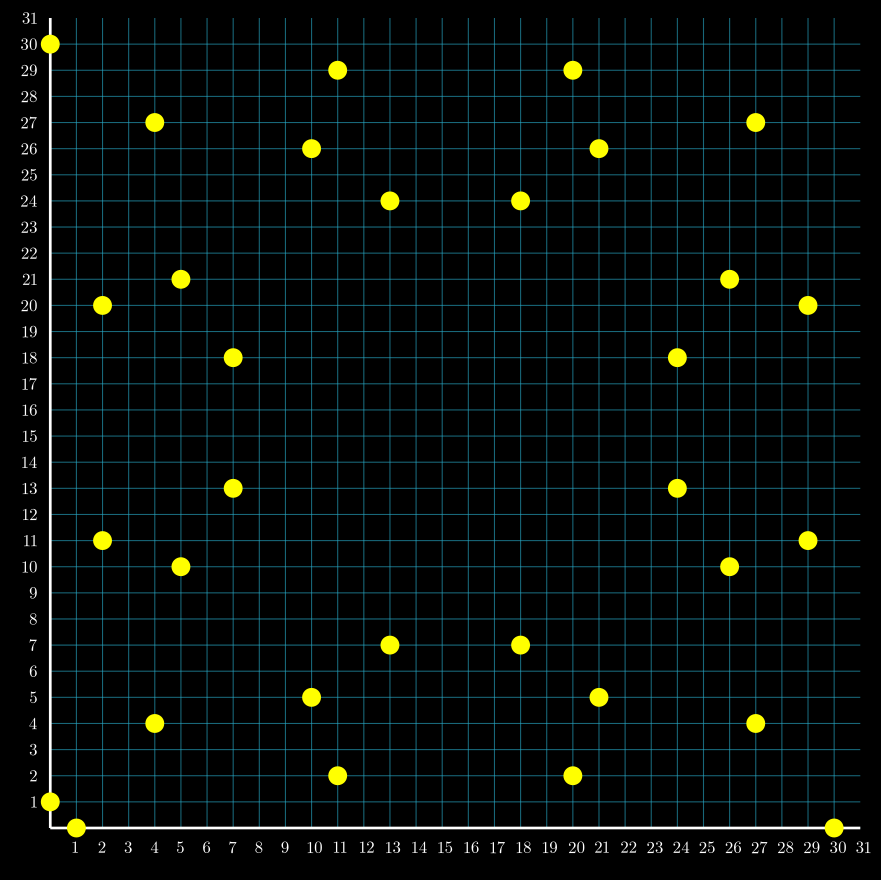
Here are a few pair examples $(x,y)$ in $\mathbb{F}_{31}^2$ that satisfy $x^2 + y^2 \equiv 1 \pmod{31}$:

• $(5,10)$ also works because $5^2 + 10^2 = 25 + 100 = 125$, and $125 \bmod 31 = 125 – 4\cdot31 = 1$.
• $(7,13)$ is also a solution: $7^2 = 49 \equiv 18$ (mod 31) and $13^2 = 169 \equiv 14$ (mod 31), so $18 + 14 = 32 \equiv 1$ (mod 31).
• $(30,0)$ demonstrates that $30 \equiv -1 \pmod{31}$, hence $(-1)^2 + 0^2 \equiv 1$ (mod 31).

To see Circle Group, let us work over $\mathbb{F}_{31}$, where the circle $C(\mathbb{F}_{31})$ has 32 points. Suppose we pick the point

$$ Q \;=\; (13,\,7).$$

We can combine $Q$ with the point $(30,0)$ via the group operation:

$$ (13,\,7) \,\cdot\,(30,\,0) \;=\; \bigl( 13 \cdot 30 – 7 \cdot 0,\;\; 13 \cdot 0 + 7 \cdot 30 \bigr) \;=\; (390,\,210) \;\equiv\; (18,\,24) \pmod{31}.$$

Indeed, one verifies

$$ 18^2 + 24^2 \;\equiv\; 324 + 576 \;\equiv\; 900 \;\equiv\; 1 \pmod{31},$$

so $(18,\,24)$ also lies on the circle $x^2 + y^2 = 1$. Meanwhile, the inverse of $Q$ is

$$ Q^{-1} \;=\; (13,\,-7)\;\equiv\;(13,\,24)\pmod{31},$$

because

$$ (13,\,7)\,\cdot\,(13,\,24) \;=\; (1,\,0).$$

Additionally, squaring map can work on the point $Q=(13,7)$. Recall that

$$ \pi(x,y) \;=\; (x,y)\,\cdot\,(x,y).$$

Hence,

$$ \pi(Q) \;=\; (13,7)\,\cdot\,(13,7) \;=\; \bigl(13\cdot 13 – 7\cdot 7,\;13\cdot 7 + 7\cdot 13\bigr) \; \;\equiv\; (27,\,27) \pmod{31}.$$

3. Subgroups of Circle Group

We have established that $C(\mathbb{F}_p)$ is a cyclic group of size $p+1$. If $p + 1$ is a power of two, say $p+1 = 2^m$, then there is a nested chain of subgroups $$G_0 \;\subset\; G_1 \;\subset\; G_2 \;\subset\; \dots \;\subset\; G_m \;=\; C(\mathbb{F}_p)$$ where each $G_k$ has order $|G_k| = 2^k$. In other words, $G_1$ is a subgroup of size 2, $G_2$ is size 4, and so on, up to $G_m = C(mathbb{F}_p)$ itself, which has size $2^m = p+1$.

For example, if $p = 31$ (so $p+1 = 32 = 2^5$), we obtain a chain $$G_0,\,G_1,\,G_2,\,G_3,\,G_4,\,G_5$$ where $G5 = C(mathbb{F}{31})$ and each $G_k$ has size $2^k$. A summary might look like this:

$k$	$\lvert G_k\rvert = 2^k$
$G_0$	1
$G_1$	2
$G_2$	4
$G_3$	8
$G_4$	16
$G_5$	32

Below, we explicitly list each subgroup in $C(\mathbb{F}_{31})$.

Size 1:  [Point(1, 0)]
Size 2:  [Point(1, 0), Point(30, 0)]
Size 4:  [Point(1, 0), Point(0, 30), Point(30, 0), Point(0, 1)]
Size 8:  [Point(1, 0), Point(4, 27), Point(0, 30), Point(27, 27), Point(30, 0), Point(27, 4), Point(0, 1), Point(4, 4)]
Size 16:  [Point(1, 0), Point(7, 13), Point(4, 27), Point(18, 24), Point(0, 30), Point(13, 24), Point(27, 27), Point(24, 13), Point(30, 0), Point(24, 18), Point(27, 4), Point(13, 7), Point(0, 1), Point(18, 7), Point(4, 4), Point(7, 18)]
Size 32:  [Point(1, 0), Point(2, 11), Point(7, 13), Point(26, 10), Point(4, 27), Point(21, 5), Point(18, 24), Point(20, 29), Point(0, 30), Point(11, 29), Point(13, 24), Point(10, 5), Point(27, 27), Point(5, 10), Point(24, 13), Point(29, 11), Point(30, 0), Point(29, 20), Point(24, 18), Point(5, 21), Point(27, 4), Point(10, 26), Point(13, 7), Point(11, 2), Point(0, 1), Point(20, 2), Point(18, 7), Point(21, 26), Point(4, 4), Point(26, 21), Point(7, 18), Point(2, 20)]

4. Python Code 1: Circle Group

We will now review the Circle Group code through the Simple Python implementation. Only the most important functions or parts are described here, and all code is available here.

Here, we define two key classes-FieldElement and CirclePoint—to handle arithmetic in the underlying finite field and group operations on the curve, respectively.

4.1 FieldElement

First, the FieldElement class defines arithmetic operations in the finite field $\mathbb{F}_{31}$, such as addition, multiplication, and inversion modulo 31. This is the foundation for all computations on the circle curve.

# Mersenne 5
MOD = 31

class FieldElement:
    def __init__(self, value):
        """Initialize a field element"""
        self.value = value % MOD

    def __add__(self, other):
        """Add two field elements"""
        return FieldElement((self.value + other.value) % MOD)

    def __mul__(self, other):
        """Multiply two field elements"""
        return FieldElement((self.value * other.value) % MOD)

    def inv(self):
        """Compute the multiplicative inverse"""
        return FieldElement(pow(self.value, MOD - 2, MOD))

    def square(self):
        """Compute the square"""
        return self * self

4.2 CirclePoint

The CirclePoint class represents points on the circle curve $x^2+y^2=1$. The add method implements the group operation, while double applies the squaring map.

class CirclePoint:
    def __init__(self, x, y):
        """Initialize a point on the circle x^2 + y^2 = 1"""
        if (x.square() + y.square()).value != 1:
            raise ValueError("Point does not lie on the circle")
        self.x = x
        self.y = y

    def add(self, other):
       """Perform group operation: (x1,y1)・(x2,y2) = (x1*x2 - y1*y2, x1*y2 + x2*y1)."""
        nx = self.x * other.x - self.y * other.y
        ny = self.x * other.y + other.x * self.y
        return CirclePoint(nx, ny)

    def double(self):
        """Apply squaring map: π(x,y) = (2*x^2 - 1, 2*x*y), since x^2 + y^2 = 1."""
        xx = self.x.square().double() - FieldElement.one()
        yy = self.x.double() * self.y
        return CirclePoint(xx, yy)

    @classmethod
    def identity(cls):
        """Return the identity element (1, 0) of the circle group."""
        return cls(FieldElement.one(), FieldElement.zero())

Then you can simulate a Circle Group operation example as described in section 2.4.

For instance, adding CirclePoint $(13, 7)$ and CirclePoint $(30, 0)$ results in Point $(18, 24)$.

p1 = CirclePoint(FieldElement(13), FieldElement(7))
p2 = CirclePoint(FieldElement(30), FieldElement(0))

# group operation
p3 = p1.add(p2)
print(f"p1・p2 = {p3}")

p1・p2 = Point(18, 24)

Doubling $p1=(13,7)$ yields $(27, 27)$

# squaring map
p1_double = p1.double()
print(f"π(p1) = {p1_double}")

π(p1) = Point(27, 27)

The inverse of $(13, 7)$ is $(13, 24)$, and adding them gives the identity $(1, 0)$

# Inverse
p1_inv = p1.inverse()
print(f"p1's inverse = {p1_inv}")
p1_plus_inv = p1.add(p1_inv)
print(f"p1・p1_inv = {p1_plus_inv}")

p1's inverse = Point(13, 24)
p1・p1_inv = Point(1, 0)

4.3 Circle Group

The function generate_subgroup generates a subgroup $G_k$ of order $2^k$. It obtains the appropriate generator from the get_nth_generator function and repeats the group operation add to construct the subgroup.

def generate_subgroup(k: int) -> list[CirclePoint]:
    """Generate a subgroup of size 2^k using the generator."""
    g_k = get_nth_generator(k)
    p = CirclePoint.identity()
    return [ (p := p.add(g_k)) if i else p
             for i in range(1 << k) ]

For example, you can get size 8 subgroup.

G3 = generate_subgroup(3)

Size 8:  [Point(1, 0), Point(4, 27), Point(0, 30), Point(27, 27), Point(30, 0), Point(27, 4), Point(0, 1), Point(4, 4)]

5. Coset, Twin-Cosets and Standard Position Cosets

Twin-Cosets and Standard Position Cosets are the domains in Circle STARKs. Let’s briefly review how domains are used in traditional STARKS before understanding the mathematical properties of twin-cosets and standard position cosets. As discussed in Section 0, traditional STARKS typically utilized multiplicative (sub)groups represented as $\mathbb{F}_p^*$ as their domains. These domains served two primary purposes.

Firstly, they acted as the evaluation domain when constructing polynomials from the computation trace via IFFT, and we have to conduct the Low Degree Extension (LDE) with the extended domain via FFT and also we construct constraint polynomials and evaluate them on LDE.

Secondly, in Low Degree Testing, particularly with FRI commitments, polynomials must be evaluated via FFT over domains that are iteratively halved during the recursive FRI folding steps.

In addition, during the FRI folding steps, as the degree of the polynomial was halved, the size of the domain also needed to be halved. Halving the domain size is central to both FRI and FFT. Keep this in mind as we proceed.

Because while the circle group itself already offers high 2-adicity, the construction of Twin-Cosets or Standard Position Cosets ensures that, during recursive squaring steps in the FFT, the evaluation domains (i.e., the Twin-Cosets or Standard Position Coset) can also be halved in size while preserving their coset structure. This is essential for enabling FFT-style operations over these domains in each level of the recursion.

5.1 Coset

Let us recall the definition of a coset in group theory. Suppose $H$ is a subgroup of a group $\mathcal{G}$, and let $Q \in \mathcal{G}$. Then the left coset of $H$ by $Q$ is the set

$$ Q \,\cdot\, H \;=\; \{\,Q \cdot h \;\mid\; h \in H\}.$$

If $Q \in H$, then $Q \cdot H = H$. Otherwise, in case of $Q \notin H$ , $Q \cdot H$ is a disjoint set from $H$, but still has the same size as $H$. This holds because if $Q \in H$, $H$’s closure under the group operation ensures $Q \cdot H = H$, while if $Q \notin H$, no element of $Q \cdot H$ can be in $H$ without implying $Q \in H$, and the bijection $h \mapsto Q \cdot h$ preserves the size.

In our particular setting, $\mathcal{G} = C(\mathbb{F}_p)$, which is cyclic of size $p+1$. From the previous section, we know there is a chain of subgroups $G_0 \subset G_1 \subset \dots \subset G_m$ with $|G_k| = 2^k$.

Hence, for instance, if we fix $G_{n-1}$ of order $2^{n-1}$, then for any point $Q$ on the circle, the coset

$$Q \,\cdot\, G_{n-1} \;=\; \bigl\{Q\cdot g \;\mid\; g\in G_{n-1}\bigr\}$$

is called a coset of $G_{n-1}$. That set will have the same cardinality $2^{n-1}$, and is disjoint from $G_{n-1}$ itself unless $Q$ already belongs to $G_{n-1}$.

5.1.1 Coset Example

Let’s illustrate this example quickly. In the case $p=31$, recall that $p+1=32=2^5$, so there is a chain of subgroups $G_1, G_2, \dots, G_5$ where $|G_1|=2$. Concretely,

$$ G_1 \;=\; \{\,(1,0),\,(30,0)\}.$$

Now take a point $Q$ not in $G_1$. For instance,

$$ Q \;=\; (2,\,11).$$

Since $Q$ is not in $G_1$, the set

$$ Q \,\cdot\, G_1 \;=\; \{\,(2,11)\cdot(1,0),\,(2,11)\cdot(30,0)\}$$

will be a distinct coset of $G_1$, disjoint from $G_1$ itself.

• $(2,11)\cdot(1,0) \;=\; (\,2\cdot1 – 11\cdot0,\;\;2\cdot0 + 11\cdot1) \;=\; (2,\,11),$

• $(2,11)\cdot(30,0) \;=\; (\,2\cdot30 – 11\cdot0,\;\;2\cdot0 + 30\cdot11) \;\equiv\; (29,\,20) \;\pmod{31}.$

Hence,

$$ Q \cdot G_1 \;=\; \{(2,\,11),\,(29,\,20)\},$$

which indeed has size 2. This is the coset of $G_1$ corresponding to $Q=(2,11)$, clearly different from the subgroup $G_1$ itself.

5.2 Twin-Cosets

We now define a twin-coset by taking the union of two cosets: $Q \cdot G_{n-1}$ and its inverse coset $Q^{-1} \cdot G_{n-1}$. Concretely, let

$$ D \;=\; \bigl(Q \,\cdot\, G_{n-1}\bigr) \;\cup\; \bigl(Q^{-1} \,\cdot\, G_{n-1}\bigr).$$

We say that $D$ is a twin-coset of size $2^n$ if the following conditions hold:

1. Disjointness The two cosets $Q \cdot G_{n-1}$ and $Q^{-1} \cdot G_{n-1}$ are disjoint.
   In practice, this disjointness is equivalent to ensuring $Q^2 \notin G_{n-1}$. This equivalence arises from the properties of cosets. If $Q^2 \in G_{n-1}$, then $Q = Q^{-1} \cdot Q^2$ would be in both $Q \cdot G_{n-1}$ and $Q^{-1} \cdot G_{n-1}$ (overlap). Conversely, if the cosets don’t overlap, then $Q$ cannot be written as $Q^{-1} \cdot g$ (for any $g \in G_{n-1}$), which implies $Q^2 \notin G_{n-1}$.

2. No fixed points under the involution $J$ A point $P$ is called a fixed point of a map $f$ if $f(P) = P$. In our case, we consider the involution $J(x,y) \;=\; \bigl(x,\;-y\bigr).$ If $D$ contained any point where $y=0$, then $J(x,0) = (x,0)$ would remain unchanged. It is a fixed point. We want to avoid having such points in $D$, because by definition a twin-coset excludes any fixed points of $J$.

Under these conditions, each coset $Q \cdot G_{n-1}$ and $Q^{-1} \cdot G_{n-1}$ has $2^{n-1}$ distinct points, giving a total of $2^n$ points in $D$. Intuitively, we merge a coset with its inverse coset, forming a domain of $2^n$ elements.

5.2.1 Twin-Coset Example

Continuing from the coset example in Section 5.1.1 (where we picked $Q=(2,11)$ not in $G_1$), let us now form a twin-coset of size $2^n = 2^2 = 4$. We already saw:

$$ Q \cdot G_1 \;=\; \{(2,\,11),\,(29,\,20)\}.$$

Next, compute $Q^{-1}=(2,\,20)$ and form the coset $Q^{-1}\cdot G_1$:

$$ Q^{-1} \,\cdot\, G_1 \;=\; \{\,(2,20)\cdot(1,0),\,(2,20)\cdot(30,0)\}$$

• $(2,20)\cdot(1,0)\;=\;\bigl(2\cdot1 \;-\;20\cdot0,\;\;2\cdot0 \;+\;1\cdot20\bigr)\;=\;(2,\,20).$

• $(2,20)\cdot(30,0)\;=\;\bigl(2\cdot30 \;-\;20\cdot0,\;\;2\cdot0 \;+\;30\cdot20\bigr)\;=\;(60,\,600)\;\equiv\;(29,\,11)\;\pmod{31}.$

Hence,

$$ Q^{-1}\cdot G_1 \;=\; \{(2,\,20),\,(29,\,11)\}.$$

Taking the union, the twin-coset is:

$$ D \;=\; \bigl(Q \cdot G_1\bigr) \;\cup\; \bigl(Q^{-1}\cdot G_1\bigr) \;=\; \{(2,\,11),\,(29,\,20)\} \;\cup\; \{(2,\,20),\,(29,\,11)\}.$$

This domain $D$ has size 4 and satisfies the twin-coset conditions: the two cosets are disjoint (since $Q^2\notin G_1$), and $D$ contains no point with $y=0$, so there are no fixed points under the involution $J(x,y)=(x,-y)$. Thus, $D$ is indeed a twin-coset of size $2^2=4$.

5.3 Standard Position Cosets

A standard position coset is a special kind of twin-coset $D$ of size $2^n$ which also coincides with a single coset of the subgroup $G_n$:

$$ D \;=\; Q \cdot G_{n-1} \;\cup\; Q^{-1}\cdot G_{n-1} \;=\; Q \cdot G_n.$$

Here, recall that $G_n$ is the unique subgroup of $C(\mathbb{F}_p)$ of order $2^n$, as introduced earlier in Section 3. We have a chain of subgroups:

$$ G_0 \subset G_1 \subset \dots \subset G_n \subset \dots \subset C(\mathbb{F}_p),$$

and each $G_k$ is of size $2^k$. So, $G_n$ contains $G_{n-1}$, and we will relate the cosets of these subgroups using a point $Q$ of order $2^{n+1}$.

Let’s unpack this step by step:

First, since $G_{n-1} \subset G_n$, we can view $G_n$ as consisting of two disjoint cosets of $G_{n-1}$, namely:

$$ G_n = G_{n-1} \cup R \cdot G_{n-1},\quad \text{for some } R \notin G_{n-1}.$$

If we now multiply this by a fixed point $Q$ of order $2^{n+1}$, we obtain:

$$ Q \cdot G_n = Q \cdot G_{n-1} \cup Q \cdot R \cdot G_{n-1}.$$

It turns out that $Q \cdot R = Q^{-1}$, so:

$$ Q \cdot G_n = Q \cdot G_{n-1} \cup Q^{-1} \cdot G_{n-1}.$$

Therefore, the coset $Q \cdot G_n$ can be written as the union of two disjoint cosets: one by $Q$, the other by $Q^{-1}$, each over the smaller subgroup $G_{n-1}$. This is exactly the definition of a twin-coset.

But not all twin-cosets arise in this way. To ensure this construction works properly, we require:

1. Disjointness: $Q^2 \notin G_{n-1}$. Otherwise, the two cosets would overlap.
2. No fixed points under involution: The resulting set $D$ must avoid points with $y = 0$, so the involution $J(x, y) = (x, -y)$ has no fixed points in $D$.
3. Correct order: $Q$ must have order $2^{n+1}$ to guarantee that $Q \cdot G_n$ spans exactly $2^n$ distinct elements.

When these are satisfied, the coset $D = Q \cdot G_n$ gives a standard position coset: a domain of size $2^n$ that is simultaneously a twin-coset and a single coset of a larger subgroup.

5.4 Hand-Computed Example: Twin-Cosets and Standard Position Cosets at $p=31$

Below, we illustrate how the notions of twin-cosets and standard position cosets apply when $p=31.$ We have $p+1=32=2^5$, so subgroups $G_1,\,G_2,\,G_3,\,G_4,\,G_5$ exist, where $|G_3|=8$ and $|G_2|=4$. We will show the standard position coset for $G_3$ that is $D=Q \cdot G_2 \;\cup\; Q^{-1} \cdot G_2=Q \cdot G_3$.

5.4.1 Twin-Coset Construction

• Setup
  Let $n=3$. Then $G_2$ has size 4. Pick a point $Q$ of order 16 (so $Q\notin G_3$, but $Q \in G_4$). Concretely, one may choose $Q = (13,\,7)$

• Forming the Twin-Coset

  $$ D= \bigl(Q \cdot G_2\bigr) \;\cup\; \bigl(Q^{-1}\cdot G_2\bigr).$$

  Since $G_2$ has the four points $(1,0)$, $(0,30)$, $(30,0)$, and $(0,1)$, each point is multiplied by $Q = (13,\,7)$ or $Q^{-1}=(13,24)$.

  1. $Q \cdot (1,0)=(13,7)$,
  2. $Q \cdot (0,30)=(7,18)$,
  3. $Q \cdot (30,0)=(18,24)$,
  4. $Q \cdot (0,1)=(24,13)$,
  5. $Q^{-1}\cdot(1,0)=(13,24)$,
  6. $Q^{-1}\cdot(0,30)=(24,18)$,
  7. $Q^{-1}\cdot(30,0)=(18,7)$,
  8. $Q^{-1}\cdot(0,1)=(7,13)$.

$$ D= \bigl(Q \cdot G_2\bigr) \;\cup\; \bigl(Q^{-1}\cdot G_2\bigr)= \{(13,7),(7,18),(18,24),(24,13),(13,24),(24,18),(18,7),(7,13)\}$$

Combining these gives 8 distinct points. No element of $D$ is fixed by $J$, so $D$ is a twin-coset of size $2^3=8$. Combining these gives 8 distinct points. No element of $D$ is fixed by $J$, so $D$ is a twin-coset of size $2^3 = 8$.

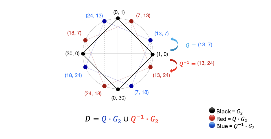
In the diagram below, 🔴 red points represent $Q \cdot G_2$ and 🔵 blue points represent $Q^{-1} \cdot G_2$. Together, they form the 8-point twin-coset $D$.

5.4.2 Checking Standard Position coset

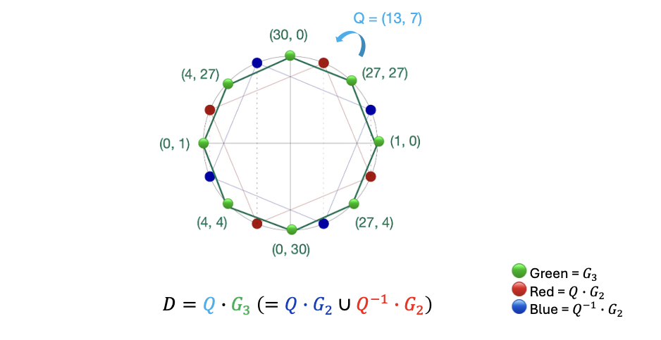
This same $D$ also equals $Q\cdot G_3$ for some subgroup $G_3$ of size 8, meaning $D$ is a standard position coset.

$G_3$ is the subgroup $\{(1,0),(4,27),(0,30),(27,27),(30,0),(27,4),(0,1),(4,4)\}$, then multiplying each element by $Q=(13,7)$ yields exactly the 8 points in $D$.

1. $Q \cdot (1,\,0) = (13,\,7)$
2. $Q \cdot (4,\,27) = (18,\,7)$
3. $Q \cdot (0,\,30) = (7,\,18)$
4. $Q \cdot (27,\,27) = (7,\,13)$
5. $Q \cdot (30,\,0) = (18,\,24)$
6. $Q \cdot (27,\,4) = (13,\,24)$
7. $Q \cdot (0,\,1) = (24,\,13)$
8. $Q \cdot (4,\,4) = (24,\,18)$

$$ Q \cdot G_3 \;=\; \{ (13,7),\,(18,7),\,(7,18),\,(7,13), (18,24),\,(13,24),\,(24,13),\,(24,18) \}.$$

Hence

$$ D= Q\cdot G_3 = Q\cdot G_2 \;\cup\; Q^{-1}\cdot G_2.$$

Because $D$ is both a twin-coset of $G_2$ and a single coset of $G_3$, we call it a standard position coset of size 8.

In the diagram below, 🟢 green points represent the subgroup $G_3$, 🔴 red and 🔵 blue points represent the two disjoint cosets $Q \cdot G_2$ and $Q^{-1} \cdot G_2$, respectively. Their union forms the twin-coset $D$, and the entire 8-point set constitutes the standard position coset $Q \cdot G_3$.

Thus, whenever $Q$ has order $2^{n+1}$, we can build a standard position coset of size $2^n$. This structure is important in Circle STARK, as it provides a neat domain of $2^n$ points even if $p-1$ is not sufficiently two-adic.

6. Python Code 2: Circle Domain

We will now review the Circle Domain code through the Simple Python implementation. The domain construction (such as twin-coset and standard position coset) is also implemented in the same Python notebook. You can run and inspect how these sets are built step-by-step.

6.1 Twin-Coset

This function generates a domain by applying group operations add to $Q$ and its inverse $Q^{-1}$ over the subgroup, ensuring symmetry and size $2^n$.

def generate_twin_coset(Q, G_n_minus_1):
    """Generate twin-coset: D = Q・G_(n-1) ∪ Q^{-1}・G_(n-1)."""
    Q_inv = Q.inverse()
    coset_Q = [Q.add(g) for g in G_n_minus_1]
    coset_Q_inv = [Q_inv.add(g) for g in G_n_minus_1]
    return coset_Q + coset_Q_inv

G2 = generate_subgroup(2)
Q = CirclePoint(FieldElement(13), FieldElement(7))
twin_cosets = generate_twin_coset(Q, G2)
print(twin_cosets)

[Point(13, 7), Point(7, 18), Point(18, 24), Point(24, 13), Point(13, 24), Point(24, 18), Point(18, 7), Point(7, 13)]

6.2 Standard Position Coset

This function generates the standard position coset by applying group operation add for $Q$ and subgroup.

def generate_standard_position_coset(Q, G_n):
    """Generate standard position coset D = Q・G_n."""
    return [Q.add(g) for g in G_n]

G3 = generate_subgroup(3)
Q = CirclePoint(FieldElement(13), FieldElement(7))
D = generate_standard_position_coset(Q, G3)

[Point(13, 7), Point(18, 7), Point(7, 18), Point(7, 13), Point(18, 24), Point(13, 24), Point(24, 13), Point(24, 18)]

This kind of code, you can check the equality of standard position coset $D \;=\;Q \,\cdot\, G_{n-1}\;\cup\;Q^{-1} \,\cdot\, G_{n-1}\;=\;Q \,\cdot\, G_n.$

D_std = generate_standard_position_coset(Q, G3)
D_twin = generate_twin_coset(Q, G2)
print("Q・G3:", D_std)
print("(Q・G2) ∪ (Q^-1・G2):", D_twin)
if set(D_std) == set(D_twin):
    print("Equal: standard position coset Q·G3 = Q·G2 ∪ Q^-1·G2")
else:
    print("Not Equal")

7. Decomposition of a Larger Standard Position Coset into Smaller Twin-Cosets

In many steps of the Circle FFT and FRI, we need to manage evaluation domains of different sizes, all of which lie on the circle curve. One key method to achieve this is Lemma 2 from the Circle STARKs paper, which ensures that a standard position coset of size $2^m$ can be broken down into smaller twin-cosets of size $2^n$ for any $n \le m$.

7.1 Statement of Lemma 2

Let $D \subset C(\mathbb{F}_p)$ be a standard position coset of size $2^m$. Then for any $n \le m$, one can decompose $D$ into twin-cosets of size $2^n$. Concretely, if

$$ D \;=\; Q \cdot G_m \quad \text{where}\quad |G_m| = 2^m,$$

then

$$ D = \bigcup_{k=0}^{\left(\frac{2^m}{2^n}\right)-1} \Bigl( Q^{4k+1} \cdot G_{n-1} \cup Q^{-(4k+1)} \cdot G_{n-1} \Bigr)$$

In simpler terms, if $D$ is a standard position coset of size $2^m$, we can slice it into smaller twin-cosets (each of size $2^n$) using powers of $Q$. This partitioning allows one to make precisely the parts of $D$ that are needed in a given step of the Circle FFT protocol.

7.2 Hand-Computed Example: Splitting a Size-$8$ standard position coset into 2 Twin-Cosets of Size $4$

Suppose $p = 31$, so $p+1 = 32 = 2^5$. We have subgroups $G_1, G_2, G_3, \dots$, where $\lvert G_3\rvert=8$.

• Our standard position coset
  Let $D = Q \cdot G_3$ with $\lvert D\rvert=8$. Here, $Q$ has order $16$, meaning $Q\notin G_3$ but $Q \cdot G_3$ forms a coset of size $8$.

$$ D= \bigl(Q \cdot G_2\bigr) \;\cup\; \bigl(Q^{-1}\cdot G_2\bigr)= Q\cdot G_3 = \{(13,7),(7,18),(18,24),(24,13),(13,24),(24,18),(18,7),(7,13)\}$$

• Goal Break $D$ into twin-cosets of size $2^n=4$. Let $n=2$, so $\lvert G_2\rvert=4$ and $\lvert G_1\rvert=2$.
  Then Lemma 2 suggests $$ D= \bigcup_{k=0}^{(8/4)-1} \Bigl( Q^{\,4k+1}\cdot G_{1} \;\cup\; Q^{-\,\bigl(4k+1\bigr)}\cdot G_{1} \Bigr).$$

  Because $8/4=2$, we have $k=0$ and $k=1$.

7.2.1 Case $k=0$

• $Q^{4\cdot0+1}=Q^1=Q$.
• $G_1=\{(1,0), (30,0)\}$.

Compute:

1. $Q\cdot(1,0) = (13,7)$
2. $Q\cdot(30,0) = (18,24)$
3. $Q^{-1}\cdot(1,0) = (13,24)$
4. $Q^{-1}\cdot(30,0) = (18,7)$

Thus, the first twin-coset has 4 distinct points.

7.2.2 Case $k=1$

• $Q^{4\cdot1+1} = Q^5$.
  That is $Q^5 = (24,13)$.
• Likewise, $Q^{-5} = (24, -13)\equiv (24,18)$.

Again, multiply each by $(1,0)$ and $(30,0)$:

1. $Q^5\cdot(1,0) = (24,13)$
2. $Q^5\cdot(30,0) = (7,18)$
3. $Q^{-5}\cdot(1,0) = (24,18)$
4. $Q^{-5}\cdot(30,0) = (7,13)$

This yields another 4 points, forming the second twin-coset of size 4.

7.2.3 Union of the Two Twin-Cosets

Taking the union of both 4-point sets (for $k=0$ and $k=1$) recovers the entire 8-element coset $D$. Hence:

$$ D=\Bigl( Q^1 \cdot G_1 \;\cup\; Q^{-1} \cdot G_1 \Bigr) \;\;\cup\;\; \Bigl( Q^5 \cdot G_1 \;\cup\; Q^{-5} \cdot G_1 \Bigr).$$

This exactly matches the statement of Lemma 2, showing how an 8-point standard position coset can be decomposed into two twin-cosets each of size 4.

7.3 Hand-Computed Example: Splitting a Size-$8$ standard position coset into 4 Twin-Cosets of Size $2$

And we can also divide this size-8 standard position coset into multiple smaller twin-cosets.

Let $n=1$, so $\lvert G_1\rvert=2$. Lemma 2 gives:

$$D = \bigcup_{k=0}^{(8/2)-1} \Bigl( Q^{4k+1}\cdot G_0 \;\cup\; Q^{-\,(4k+1)}\cdot G_0 \Bigr).$$

Since $G_0 = \{(1,0)\}$, each twin-coset has 2 points:

• $k=0$: $\{Q^1 \cdot G_0 = Q, Q^{-1} \cdot G_0 = Q^{-1}\}$ $=\{(13, 7), (13, 24)\}$
• $k=1$: $\{Q^5 \cdot G_0 = Q^5, Q^{-5} \cdot G_0 = Q^{-5}\}$$=\{(24, 13), (24, 18)\}$  
• $k=2$: $\{Q^9 \cdot G_0 = Q^9, Q^{-9} \cdot G_0 = Q^{-9}\}$$=\{(18, 24), (18, 7)\}$  
• $k=3$: $\{Q^{13} \cdot G_0 = Q^{13}, Q^{-13} \cdot G_0 = Q^{-13}\}$$=\{(7, 18), (7, 13)\}$

$D = \{(13,7),(13,24)\} \cup \{(24,13),(24,18)\} \cup \{(18,24),(18,7)\} \cup \{(7,18),(7,13)\}$

This decomposes $D$ into four twin-cosets of size $2$.

8. Squaring Map Halves a Twin-Coset

While Lemma 2 focuses on splitting large cosets into smaller twin-cosets, Lemma 3 exploits a squaring map to halve the size of a twin-coset. This process is used for the domain halving steps in Circle FFT, where we iteratively reduce the domain size.

8.1 Statement of Lemma 3

This lemma appears in the Circle STARKs paper, where it is used to formalize the recursive domain halving enabled by the squaring map.

Suppose $D$ is a twin-coset of size $2^n$ (with $n \ge 2$). Then applying the squaring map $\pi(x,y) = (x^2 – y^2,\,2xy)$ transforms $D$ into another twin-coset $\pi(D)$ of size $2^{n-1}$. Moreover, if $D$ was a standard position coset, then $\pi(D)$ also remains a standard position coset.

Intuitively, $\pi$ is a group endomorphism, and it maps a subgroup $G_{n-1}$ into $G_{n-2}$. Hence, a twin-coset of size $2^n$ naturally yields another twin-coset of size $2^{n-1}$.

8.1.1 Abstract View of Lemma 3’s Proof

Let $D$ be a twin-coset of size $2^n$, which in an abstract notation means

$$ D = Q \cdot G_{n-1} \;\cup\; Q^{-1}\cdot G_{n-1},$$

where $|G_{n-1}| = 2^{n-1}$. In particular, $\pi$ maps the subgroup $G_{n-1}$ onto $G_{n-2}$ due to a group endomorphism.

$$ \pi(D) \;=\; \pi\!\Bigl(Q \cdot G_{n-1} \cup Q^{-1}\cdot G_{n-1}\Bigr)= \bigl(\pi(Q) \cdot G_{n-2}\bigr) \;\cup\; \bigl(\pi(Q)^{-1} \cdot G_{n-2}\bigr).$$

This is exactly the definition of a twin-coset in the subgroup $G_{n-2}$, which has size $2^{n-2}$. Accordingly, $\pi(D)$ is itself a twin-coset of size $2^{n-1}$.

If $D$ was originally a standard position coset, then applying $\pi$ preserves that standard position property, because $\pi(G_n) = G_{n-1}$. Thus $\pi(D)$ is again a standard position coset, but now of size $2^{n-1}$.

8.2 Hand-Computed Example (Halving a Size-$8$ Twin-Coset to Size $4$)

Assume $p=31$ and let $D$ be a twin-coset of size $2^3=8$. Concretely,

$$ D = Q\cdot G_2 \;\cup\; Q^{-1}\cdot G_2 \quad\text{with}\quad Q=(13,7).$$

Since $\lvert G_2\rvert=4$, we have $\lvert D\rvert=8$. We check how $\pi$ affects $D$:

8.2.1 Computing $\pi(Q)$ and $\pi(Q^{-1})$

$$ \pi(Q)= \bigl(13^2 – 7^2,\;2\cdot13\cdot7\bigr)= (27,\,27),$$ $$ \pi(Q^{-1})= (27,\,4).$$

8.2.2 Applying $\pi$ to $D$

The subgroup $G_1$ has size 2, say $G_1 = \{(1,0), (30,0)\}$. By Lemma 3, $$pi(D) = bigl(pi(Q)cdot G_1bigr) ;cup; bigl(pi(Q)^{-1}cdot G_1bigr).

$$ – $\pi(Q)\cdot(1,0) = (27,27)$ – $\pi(Q)\cdot(30,0) = (4,4)$ – $\pi(Q^{-1})\cdot(1,0) = (27,4)$ – $\pi(Q^{-1})\cdot(30,0) = (4,27)$ $$

{(27,27),, (4,4)} ;cup; {(27,4),, (4,27)}

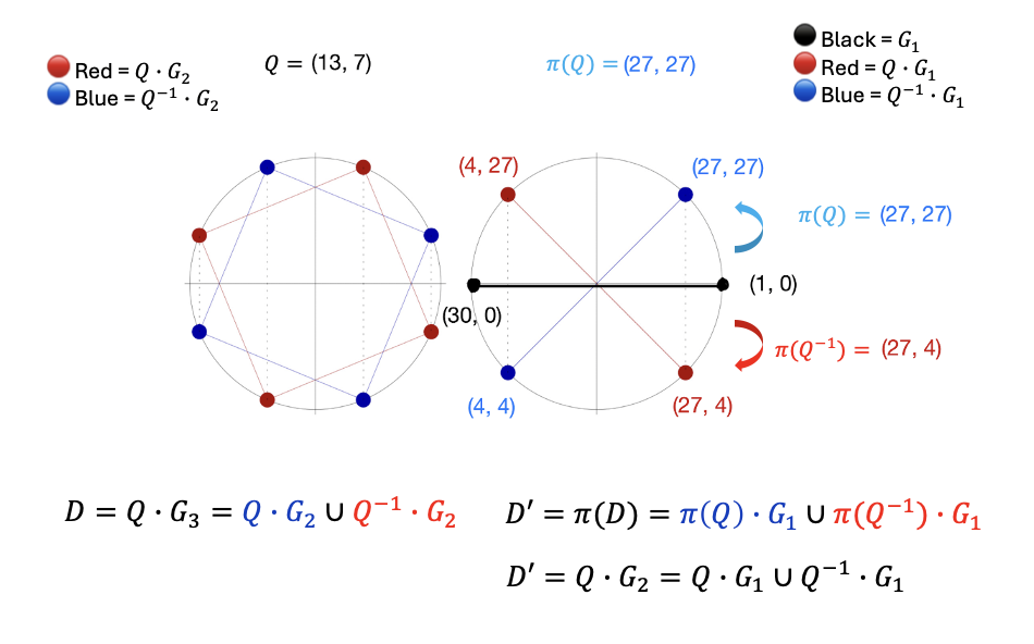
$$ which is a twin-coset of size 4. Thus, $\pi$ halves $D$ from 8 elements to 4, exactly as Lemma 3 states. Repeated application of $\pi$ continues to shrink the domain in powers of 2, playing a critical role in the recursive structure of the Circle FFT. In the diagram below: – The left circle shows the original twin-coset $D = Q \cdot G_2 \cup Q^{-1} \cdot G_2$, where 🔴 red = $Q \cdot G_2$ and 🔵 blue = $Q^{-1} \cdot G_2$. – The right circle shows the halved twin-coset $\pi(D)$, where 🔵 blue = $\pi(Q) \cdot G_1$ and 🔴 red = $\pi(Q^{-1}) \cdot G_1$. – ⚫ Black points mark the subgroup $G_1 = \{(1, 0), (30, 0)\}$. This visual illustrates how $\pi$ maps the original domain of size $2^3 = 8$ into a new twin-coset of size $2^2 = 4$ via group endomorphism.  ## 9. What We Built in Part 1 In this article, we focused on how the circle curve $x^2 + y^2 = 1$ over $\mathbb{F}_p$ can be turned into a cyclic group of size $p + 1$, and we discussed twin-cosets and standard position cosets with concrete examples. We also showed two key techniques: one for splitting a larger standard position coset into smaller twin-cosets, and another for halving the size of a twin-coset by applying the squaring map. Together, these techniques let us reshape domains of size $2^n$ at will. In the next part, we will dive deeper into the Circle FFT itself, showing how these $2^n$-sized domains—together with the ability to split or halve them—enable fast polynomial evaluation and interpolation, even when $p – 1$ is not sufficiently two-adic. ## References – Circle STARKs https://eprint.iacr.org/2024/278 – Plonky3 https://github.com/Plonky3/Plonky3 – ZK11: Circle STARKs – Ulrich Haböck & Shahar Papini – Circle STARKs: Part I, Mersenne https://blog.zksecurity.xyz/posts/circle-starks-1/ – Why I’m Excited By Circle Stark And Stwo

Why I’m Excited By Circle Stark And Stwo

– Exploring circle STARKs https://vitalik.eth.limo/general/2024/07/23/circlestarks.html – An introduction to circle STARKs https://blog.lambdaclass.com/an-introduction-to-circle-starks/ – Yet another circle STARK tutorial https://research.chainsafe.io/blog/circle-starks/ – Deep dive into Circle-STARKs FFT https://ihagopian.com/posts/deep-dive-into-circle-starks-fft – Coset’s Circle STARKs lecture videos – Ethereum/research/circlestark(Python implementation) https://github.com/ethereum/research/tree/master/circlestark – Rust Implementation Demo of Circle Domain and Circle FFT https://github.com/0xxEric/CircleFFT – STARKの原理 https://zenn.dev/qope/articles/8d60f77e3a7630 ## Appendix Below, we introduce the Projective vs Affine view of the circle curve, and then explain why Circle STARKs specifically chooses primes $p \equiv 3 \pmod{4}$ to avoid projective complications like points at infinity. ### A.1 Projective and Affine In an affine plane over $\mathbb{F}_p$, a point is simply written as $(x,y)$ with $x,y \in \mathbb{F}_p$. By contrast, in the projective plane $\mathbb{P}^2(\mathbb{F}_p)$, each point is denoted by $(X : Y : Z)$, but all nonzero scalar multiples represent the same location. Formally,$$

(X : Y : Z) ;equiv; (lambda X : lambda Y : lambda Z)quad (lambda neq 0).

$$ – When $Z \neq 0$, we can re-scale by dividing each coordinate by $Z$, giving an affine point $\bigl(X/Z,\;Y/Z\bigr)$. – When $Z=0$, we get a point at infinity, which has no affine counterpart. ### A.2 Why Avoid Points at Infinity? To see how points at infinity arise, rewrite $x^2 + y^2 = 1$ in projective form:$$

X^2 + Y^2 ;=; Z^2.

Here, if $Z \neq 0$, we regard $x = X/Z$ and $y = Y/Z$, so $x^2 + y^2 = 1$ becomes $X^2 + Y^2 = Z^2$. A point at infinity is any solution with $Z=0$. Whether such solutions exist depends on whether $-1$ is a square in $\mathbb{F}_p$: – For example, if $p \equiv 1 \pmod{4}$, then $-1$ is a square in $\mathbb{F}_p$. Concretely, there is some $a$ with $a^2 \equiv -1 \pmod{p}$, implying $X^2 + Y^2 \equiv 0 \pmod{p}$ can have nonzero $(X,Y)$ at $Z=0$. This yields extra infinite points on the circle, complicating group operations and implementation. Example: $p=5$ – Here, $-1 \equiv 4$ in $\mathbb{F}_5$, and $4$ is indeed $(2^2)$. – So $X^2 + Y^2 \equiv 0 \pmod{5}$ admits nonzero $(X,Y)$ at $Z=0$, giving two points at infinity. – The affine equation $x^2 + y^2=1$ has exactly four affine solutions: $$\{(0,1),\,(0,4),\,(1,0),\,(4,0)\}.$$ – And the projective points at infinity are $\{(2:1:0), (3:1:0)\}$, there are $6$ solutions in total — matching $p+1=6$ (affine $4$ + infinite $2$). – If $p \equiv 3 \pmod{4}$, then $-1$ is not a square in $\mathbb{F}_p$. Consequently, $X^2 + Y^2 \equiv 0 \pmod{p}$ has no nonzero solutions at $Z=0$. We get no points at infinity, and all solutions remain affine. Example: $p=3$ – Since $-1 \equiv 2 \pmod{3}$ is not a square (we have $1^2 \equiv 1$ and $2^2 \equiv 1$), no $(X,Y)$ satisfy $X^2+Y^2\equiv0$ at $Z=0$. – The equation $x^2 + y^2=1$ then has only affine solutions. Checking $x,y \in \{0,1,2\}$ yields: $$\{(0,1),\,(0,2),\,(1,0),\,(2,0)\}, $$ for a total of $4$ solutions, matching $p+1=4$. In Circle STARK, we specifically choose $p \equiv 3 \pmod{4}$ so that $-1$ is not a square in $\mathbb{F}_p$. This ensures our circle $x^2 + y^2=1$ has no infinite (projective) points, keeping every solution in affine coordinates and avoids the complexities of handling points at infinity.