Elliptic Curves over Finite Fields

What do elliptic curves in finite fields look like?

It’s easy to visualize smooth elliptic curves, but what do elliptic curves over a finite field look like?

The following is a plot of $y² = x³ + 3 \pmod {23}$

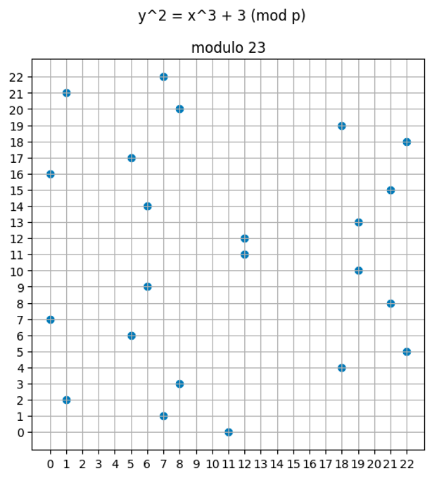
Because we only allow integer inputs (more specifically, finite field elements), we are not going to obtain a smooth plot.

Not every $x$ value will result in an integer for the $y$ value when we solve the equation, so no point will be present at that value for $x$. You can see such gaps in the plot above.

Code to generate this plot will be provided later.

The prime number changes the plot dramatically

Here are some plots of $y² = x³ + 3$ done over modulo 11, 23, 31, and 41 respectively. The higher the modulus, the more points it holds, and the more complex the plot appears to be.

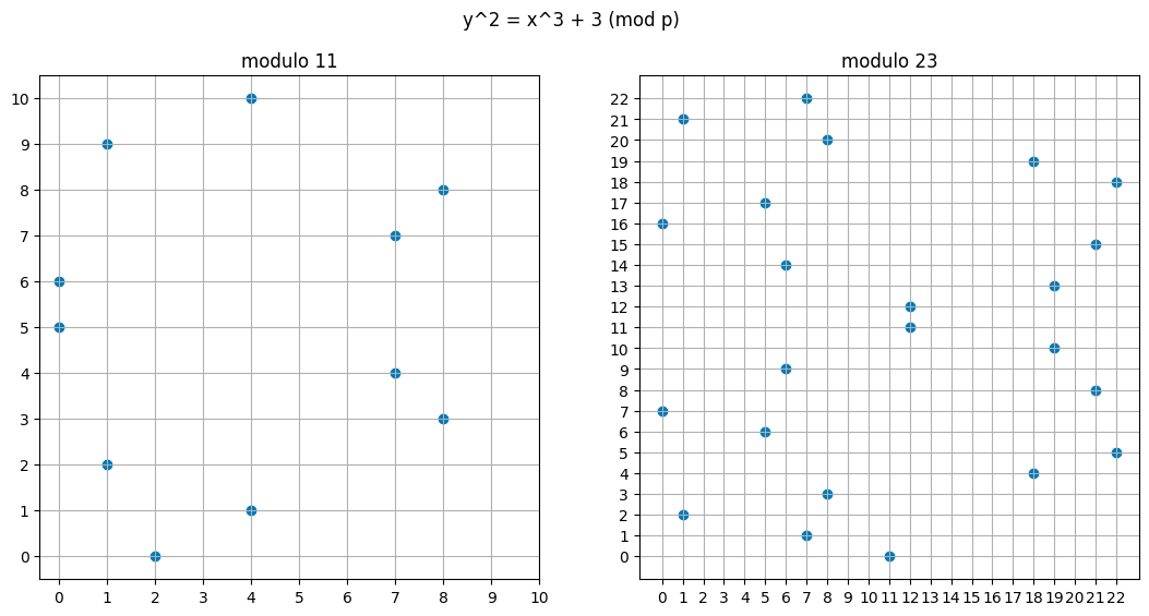
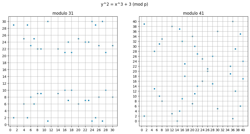
We established in the previous article that elliptic curve points with the “connect and flip” operation are a group. When we do this over a finite field, it remains a group, but it becomes a cyclic group, which is tremendously useful for our application. Why it is cyclic unfortunately will require some very involved math, so you’ll just have to accept that for now. But this should not be too surprising. We have a finite number of points, so generating each point by carrying out $(x + 1)G, (x + 2)G, … (x + \text{order} – 1)G$ should at least seem plausible.

In the application of cryptography, $p$ needs to be large. In practice, it is over 200 bits. We will revisit this in a later section.

Background

Field element

We’re going to say “field element” a lot in this article, and hopefully from our previous tutorials (especially on finite fields) you are comfortable with that term already. But if not, it is a positive integer that is inside a modulo operation.

That is, if we do addition modulo 11, then the finite field elements from that set is $\set{0,1,…,9,10}$. It isn’t correct to say “integers” even though that’s the data type we will use in our Python examples. You cannot have a negative field element (although integers can be negative) when doing addition modulo a prime number. A “negative” number in a finite field is simply the additive inverse of another number, that is, a number that when summed together results in zero. For example, in a finite field of modulo 11, 4 can be considered “-7” because $7 + 4 \pmod {11}$ is $0$, in a comparative sense to how 7 + (-7) is zero for regular numbers.

Over the field of rational numbers, multiplication has the identity element of 1, and the inverse of a number is simply the numerator and the denominator flipped. For example, 500/303 is the inverse of 303/500 because if you multiply them, you get 1.

In a finite field, the inverse of an element is the number you multiply it with to get the finite field element 1. For example, in modulo 23, 6 is the inverse of 4 because when you multiply them together modulo 23, you get 1. When the order of the field is prime, every number except zero has an inverse.

Cyclic Groups

A cyclic group is a group such that every element can be computed by starting with a generator element and repeatedly applying the group’s binary operator.

A very simple example is integers modulo 11 under addition. If your generator is 1, and you keep adding the generator to itself, you can generate every element in the group from 0 to 10.

Saying a elliptic curve points form a cyclic group (under elliptic curve addition) means we can represent every number in a finite field as an elliptic curve point and add them together just like we would regular integers in a finite field.

That is,

$5 + 7 \pmod p$ is homomorphic to $5G + 7G$

Where G is the generator of the elliptic curve cyclic group.

This is only true of elliptic curves over finite fields that have a prime number of points, which are the kinds of curves we use in practice. This is something we’ll revisit later.

BN128 formula

The BN128 curve, which is used by the Ethereum precompiles to verify ZK proofs, is specified as follows:

$$ p = 21888242871839275222246405745257275088696311157297823662689037894645226208583 $$

$$ y² = x³ + 3 \pmod p $$

Here $p$ is the field modulus.

The field_modulus should not be confused with the curve order, which is the number of points on the curve.

For the bn128 curve, the curve order is as follows:

from py_ecc.bn128 import curve_order
# 21888242871839275222246405745257275088548364400416034343698204186575808495617
print(curve_order)

The field modulus is very large, which makes experimenting with it unwieldy. In the next section, we’ll build up an intuition for elliptic curve points in finite fields using the same formula, but with a smaller modulus.

Generating elliptic curve cyclic group $y² = x³ + 3 \pmod {11}$

To solve the equation above, and determine which $(x, y)$ points are on the curve, we’ll need to compute $\sqrt{(x³ + 3)} \pmod {11}$.

Modular square roots

We use the Tonelli Shanks Algorithm to compute modular square roots. You can read up on how the algorithm works if you are curious, but for now you can treat it as a black box that computes the mathematical square root of a field element over a modulus, or lets you know if the square root does not exist.

For example, the square root of 5 modulo 11 is 4 $(4 \times 4 \mod 11 = 5)$, but there is no square root of 6 modulo 11. (The reader is encouraged to discover this is true via brute force).

Square roots often have two solutions, a positive and a negative one. Although we don’t have numbers with a negative sign in a finite field, we still have a notion of “negative numbers” in the sense of having an inverse.

You can find code online to implement the algorithm described above, but to avoid putting large chunks of code in this tutorial, we will install a Python library instead.

python3 -m pip install libnum

After installing libnum, we can run the following code to demonstrate its use.

from libnum import has_sqrtmod_prime_power, sqrtmod_prime_power

# the functions take arguments# has_sqrtmod_prime_power(n, field_mod, k), where n**k,
# but we aren't interested in powers in modular fields, so we set k = 1
# check if sqrt(8) mod 11 exists
print(has_sqrtmod_prime_power(8, 11, 1))
# False

# check if sqrt(5) mod 11 exists
print(has_sqrtmod_prime_power(5, 11, 1))
# True

# compute sqrt(5) mod 11
print(list(sqrtmod_prime_power(5, 11, 1)))
# [4, 7]

assert (4 ** 2) % 11 == 5
assert (7 ** 2) % 11 == 5

# we expect 4 and 7 to be inverses of each other, because in "regular" math, the two solutions to a square root are sqrt and -sqrt
assert (4 + 7) % 11 == 0

Now that we know how to compute modular square roots, we can iterate through values of $x$ and compute $y$ from the formula $y² = x³ + b$. Solving for $y$ is just a matter of taking the modular square root of both sides (if it exists) and saving the resulting $(x, y)$ pairs so we can plot them later.

Let’s create a simple plot of an elliptic curve

$$y² = x³ + 3 \pmod {11}$$

import libnum
import matplotlib.pyplot as plt

def generate_points(mod):
    xs = []
    ys = []
    def y_squared(x):
        return (x**3 + 3) % mod

    for x in range(0, mod):
        if libnum.has_sqrtmod_prime_power(y_squared(x), mod, 1):
            square_roots = libnum.sqrtmod_prime_power(y_squared(x), mod, 1)

            # we might have two solutions
            for sr in square_roots:
                ys.append(sr)
                xs.append(x)
    return xs, ys


xs, ys = generate_points(11)
fig, (ax1) = plt.subplots(1, 1);
fig.suptitle('y^2 = x^3 + 3 (mod p)');
fig.set_size_inches(6, 6);
ax1.set_xticks(range(0,11));
ax1.set_yticks(range(0,11));
plt.grid()
plt.scatter(xs, ys)
plt.plot();

The result of the plot is shown below:

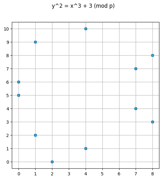
Some observations:

• There won’t be any x or y values greater than or equal to the modulus we use
• Just like the real-valued plot, the modular one “appears symmetric”

Elliptic curve point addition

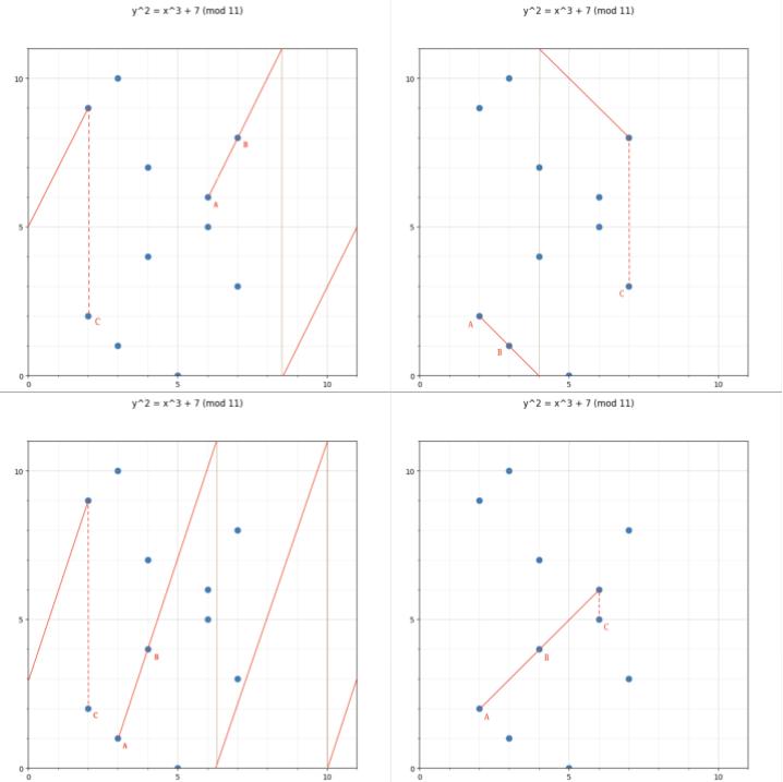
Even more interestingly, our “connect the dots and flip” operation to compute elliptic curves still works!

But given that we are doing this over a finite field, this should not be surprising. Our formulas over real numbers use the normal field operations of addition and multiplication. Although we use square roots to determine if a point is on the curve, and square roots are not a valid field operator, we do not use square roots to compute the addition and doubling of points.

The reader can verify this by picking two points from the plots above, then plugging them into the code below to add points and seeing they always land on another point (or the point on infinity if the points are inverses of each other). These formulas are taken from the Wikipedia page on elliptic curve point multiplication.

def double(x, y, a, p):
    lambd = (((3 * x**2) % p ) *  pow(2 * y, -1, p)) % p
    newx = (lambd**2 - 2 * x) % p
    newy = (-lambd * newx + lambd * x - y) % p
    return (newx, newy)

def add_points(xq, yq, xp, yp, p, a=0):
    if xq == yq == None:
        return xp, yp
    if xp == yp == None:
        return xq, yq

    assert (xq**3 + 3) % p == (yq ** 2) % p, "q not on curve"
    assert (xp**3 + 3) % p == (yp ** 2) % p, "p not on curve"

    if xq == xp and yq == yp:
        return double(xq, yq, a, p)
    elif xq == xp:
        return None, None

    lambd = ((yq - yp) * pow((xq - xp), -1, p) ) % p
    xr = (lambd**2 - xp - xq) % p
    yr = (lambd*(xp - xr) - yp) % p
    return xr, yr

Here are some visualizations of what “connect and flip” looks like in a finite field:

Every elliptic curve point in a cyclic group has a “number”

A cyclic group, by definition, can be generated by repeatedly adding the generator to itself.

Let’s use a real example of $y² = x³ + 3 \pmod {11}$ with the generator point being $(4, 10)$.

Using the Python functions above, we can start with the point $(4, 10)$ and generate every point in the group:

# for our purposes, (4, 10) is the generator point G
next_x, next_y = 4, 10print(1, 4, 10)
points = [(next_x, next_y)]
for i in range(2, 12):
    # repeatedly add G to the next point to generate all the elements
    next_x, next_y = add_points(next_x, next_y, 4, 10, 11)
    print(i, next_x, next_y)
    points.append((next_x, next_y))

The output will be

0 4 10
1 7 7
2 1 9
3 0 6
4 8 8
5 2 0
6 8 3
7 0 5
8 1 2
9 7 4
10 4 1
11 None None
12 4 10 # note that this is the same point as the first one

Observe that $(\text{order} + 1)G = G$. Just like modular addition, when we “overflow”, the cycle starts over.

Here, None means the point at infinity, which is indeed part of the group. Adding the point at infinity to the generator returns the generator, as that is how the identity element is supposed to behave.

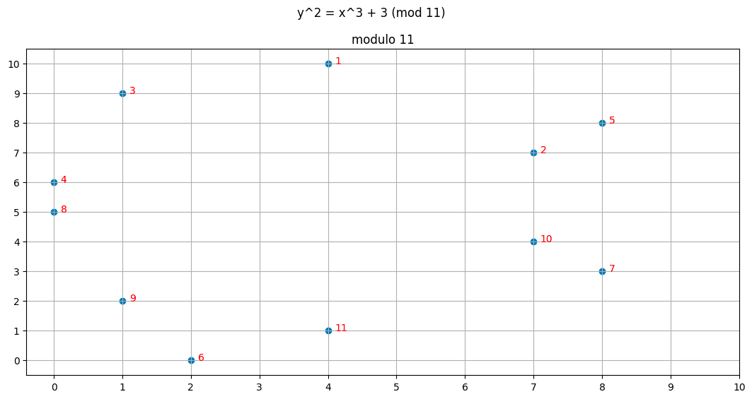
We can assign each point a “number” based on how many times we added the generator to itself to arrive at that point.

We can use the following code to plot the curve and assign a number next to it

xs11, ys11 = generate_points(11)

fig, (ax1) = plt.subplots(1, 1);
fig.suptitle('y^2 = x^3 + 3 (mod 11)');
fig.set_size_inches(13, 6);

ax1.set_title("modulo 11")
ax1.scatter(xs11, ys11, marker='o');
ax1.set_xticks(range(0,11));
ax1.set_yticks(range(0,11));
ax1.grid()

for i in range(0, 11):
    plt.annotate(str(i+1), (points[i][0] + 0.1, points[i][1]), color="red");

The red text can be thought of as starting with the identity element, and how many times we added the generator to it.

Point inverses are still vertically symmetric

Here is an interesting observation: note that points that share the same x-value add up to 12, which corresponds to the identity element $(12 \mod 12 = 0)$. If we add the point $(4, 1)$, which is point 11 in our plot to $(4, 10)$, we will get the point at in infinity, which would be the 12th element in the group.

The order is not the modulus

In this example, the order of the group is 12 (total number of elliptic curve points in our group), despite the formula for the elliptic curve being modulo 11. This will be stressed several times, but you should NOT assume that the modulus in the elliptic curve is the group order. However, you can estimate the curve’s order range from the field modulus itself using Hasse’s Theorem.

If the number of points is prime, then the addition of points behaves like a finite field

In the plot above, there are 12 points (including 0). Addition modulo 12 is not a finite field because 12 is not prime.

However, if we pick our parameters for the curve carefully, we can create an elliptic curve where the points correspond to elements in a finite field. That is, the order of the curve equals the order of the finite field.

For example, $y^2 = x^3 + 7 \pmod {43}$ creates a curve with 31 points total as can be seen in the plot below:

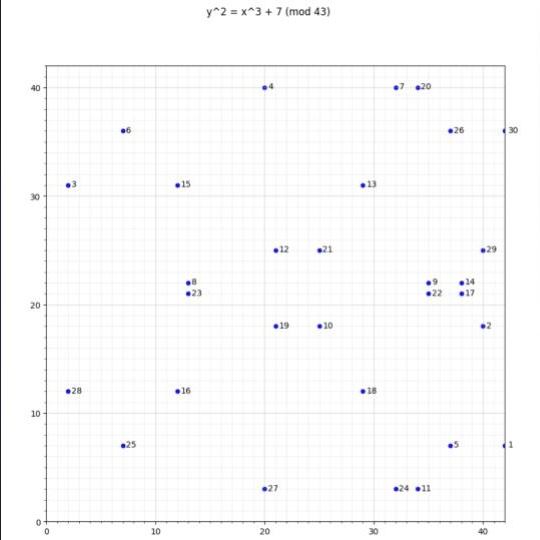
When the order of the curve matches the order of the finite field every operation you do in the finite field has a homomorphic equivalent in the elliptic curve.

To go from a finite field to an elliptic curve, we we pick one point (arbitrarily) to be the generator, then we multiply the element in the finite field by the generator.

Multiplication is really repeated addition

There is no such thing as elliptic curve point multiplication. When we say “scalar multiplication” we really mean repeated addition. You cannot take two elliptic curve points and multiply them together (well, you sort of can with bilinear pairings, but that’s something we will get to later).

When we use the Python library to do multiply(G1, x), this is really the same as G1 + G1 + … + G1 x times. Under the hood, we don’t actually self-add that many times, we use some clever shortcuts with point doubling to complete the operation in logarithmic time.

For example, if we wanted to compute 135G, we would really compute the following values efficiently using point doubling, cache them,

G, 2G, 4G, 8G, 16G, 32G, 64G, 128G

…then sum up 128G + 4G + 2G + G = 135G.

When we say 5G + 6G = 11G, we are essentially just adding G to itself 11 times. Using the shortcut illustrated above, we can compute 11G with a logarithmic number of computations, but at the end of the day, it’s just repeated addition.

Python bn128 library

The library the EVM implementation pyEVM uses for the elliptic curve precompiles is py_ecc, and we will be relying on that library heavily. The code below shows what the generator points looks like, and also shows some addition and scalar multiplication.

Here is what a G1 point looks like:

from py_ecc.bn128 import G1, multiply, add, eq, neg

print(G1)
# (1, 2)

print(add(G1, G1))
# (1368015179489954701390400359078579693043519447331113978918064868415326638035, 9918110051302171585080402603319702774565515993150576347155970296011118125764)

print(multiply(G1, 2))
#(1368015179489954701390400359078579693043519447331113978918064868415326638035, 9918110051302171585080402603319702774565515993150576347155970296011118125764)

# 10G + 11G = 21G
assert eq(add(multiply(G1, 10), multiply(G, 11)), multiply(G1, 21))

Although the numbers are large and hard to read, we can see adding a point to itself results in the same value as “multiplying” a point by 2. The two points above are clearly the same point. The tuple is still an $(x, y)$ pair, just over a very large domain.

The number printed above is huge for a reason. We do not want attackers to be able to take an elliptic curve point and compute the field element that generated it. If the order of our cyclic group is too small, then the attacker can just brute force it.

Here is a plot of the first 1000 points:

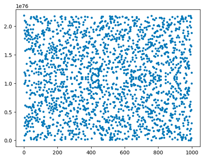
And this is the code to generate the plot above:

import matplotlib.pyplot as plt
from py_ecc.bn128 import G1, multiply, neg
import math
import numpy as np
xs = []
ys = []
for i in range(1,1000):
    xs.append(i)
    ys.append(int(multiply(G1, i)[1]))
    xs.append(i)
    ys.append(int(neg(multiply(G1, i))[1]))
plt.scatter(xs, ys, marker='.')

This may look scary, but the only difference from what we did in the previous section is using a much larger modulus and a different point for the generator.

Addition in the library

The py_ecc library makes point addition convenient for us, and the syntax should be self-explanatory:

from py_ecc.bn128 import G1, multiply, add, eq

# 5 = 2 + 3
assert eq(multiply(G1, 5), add(multiply(G1, 2), multiply(G1, 3)));

Addition in a finite field is homomorphic to addition among elliptic curve points (when their order is equal). Because of the discrete logarithm, another party can add elliptic curve points together without knowing which field elements generated those points.

At this point, hopefully the reader has a good intuition for adding elliptic curve points together, both theoretically and practically, because modern zero knowledge algorithms rely heavily on this..

Implementation detail about the homomorphism between modular addition and elliptic curve addition

We need to make a careful distinction between terminologies here:

The field modulus is the modulo we do the curve over. The curve order is the number of points on the curve.

If you start with a point $R$ and add the curve order $o$, you will get $R$ back. If you add the field modulus, you will get a different point.

from py_ecc.bn128 import curve_order, field_modulus, G1, multiply, eq

x = 5 # chosen randomly
# This passes
assert eq(multiply(G1, x), multiply(G1, x + curve_order))

# This fails
assert eq(multiply(G1, x), multiply(G1, x + field_modulus))

The implication of this is that (x + y) mod curve_order == xG + yG.

x = 2 ** 300 + 21
y = 3 ** 50 + 11

# (x + y) == xG + yG
assert eq(multiply(G1, (x + y)), add(multiply(G1, x), multiply(G1, y)))

Even though the x + y operation will clearly “overflow” over the curve order, this doesn’t matter. Just like in a finite field, this is the behavior we expect. The elliptic curve multiplication is implicitly executing the same operation as taking the modulus before doing the multiplication.

In fact, we don’t even need to do the modulus if we only care about positive numbers, the following identity also holds:

x = 2 ** 300 + 21
y = 3 ** 50 + 11

assert eq(multiply(G1, (x + y) % curve_order), add(multiply(G1, x), multiply(G1, y)))

However, if we do the finite math modulo with the wrong number (some number other than the curve order), the equality will break if we “overflow”

x = 2 ** 300 + 21
y = 3 ** 50 + 11 # these values are large enough to overflow:

assert eq(multiply(G1, (x + y) % (curve_order - 1)), add(multiply(G1, x), multiply(G1, y))), "this breaks"

Encoding rational numbers

When we take the modulus, we are able to encode a concept of division.

For example, we cannot do the following using regular integers.

# this throws an exception
eq(add(multiply(G1, 5 / 2), multiply(G1, 1 / 2), multiply(G1, 3)

However, in a finite field, 1/2 can be meaningfully computed as the multiplicative inverse of 2. Therefore, 5 / 2 can be encoded as $5 \cdot \mathsf{inv}(2)$.

Here’s how we can do it in Python:

five_over_two = (5 * pow(2, -1, curve_order)) % curve_order
one_half = pow(2, -1, curve_order)

# Essentially 5/2 = 2.5# 2.5 + 0.5 = 3
# but we are doing this in a finite field
assert eq(add(multiply(G1, five_over_two), multiply(G1, one_half)), multiply(G1, 3))

Associativity

We know groups are associative, so we expect the following identity to be true in general:

x = 5
y = 10
z = 15

lhs = add(add(multiply(G1, x), multiply(G1, y)), multiply(G1, z))

rhs = add(multiply(G1, x), add(multiply(G1, y), multiply(G1, z)))

assert eq(lhs, rhs)

The reader is encouraged to try different values of x, y, and z for themselves.

Every element has an inverse

The py_ecc library supplies us with the neg function which will provide the inverse of a given element by flipping it over the y-axis (in a finite field). The library encodes the “point at infinity” as a Python None.

from py_ecc.bn128 import G1, multiply, neg, is_inf, Z1

# pick a field element
x = 12345678# generate the point
p = multiply(G1, x)

# invert
p_inv = neg(p)

# every element added to its inverse produces the identity elementassert is_inf(add(p, p_inv))

# Z1 is just None, which is the point at infinity
assert Z1 is None

# special case: the inverse of the identity is itself
assert eq(neg(Z1), Z1)

As is the case with elliptic curves over real numbers, the inverse of an elliptic curve point has the same x value, but the y value is the inverse.

from py_ecc.bn128 import G1, neg, multiply

field_modulus = 21888242871839275222246405745257275088696311157297823662689037894645226208583
for i in range(1, 4):
    point = multiply(G1, i)
    print(point)
    print(neg(point))
    print('----')

    # x values are the same
    assert int(point[0]) == int(neg(point)[0])

    # y values are inverses of each other, we are adding y values
    # not ec points
    assert int(point[1]) + int(neg(point)[1]) == field_modulus

Every element can be generated by a generator

When we are dealing with over $2^{200}$ points, this is not possible to verify by brute force. However, consider the fact that eq(multiply(G1, x), multiply(G1, x + order)) is always true. That means we are able to generate up to order points, then it cycles back to where it started.

What about optimized_bn128?

Examining the library, you will see an implementation called optimized_bn128. If you benchmark the execution time, you will see this version runs much quicker, and it is the implementation used by pyEvm. For educational purposes however, it is preferable to use the non-optimized version as it structures the points in a more intuitive way (the usual x, y tuple). The optimized version structures EC points as 3-tuples, which are harder to interpret.

from py_ecc.optimized_bn128 import G1, multiply, neg, is_inf, Z1
print(G1)
# (1, 2, 1)

Basic zero knowledge proofs with elliptic curves

Consider this rather trivial example:

Claim: “I know two values $x$ and $y$ such that $x + y = 15$”

Proof: I multiply x by G1 and y by G1 and give those to you as A and B.

Verifier: You multiply 15 by G1 and check that A + B == 15G1.

Here it is in Python:

from py_ecc.bn128 import G1, multiply, add

# Prover
secret_x = 5
secret_y = 10

x = multiply(G1, 5)
y = multiply(G1, 10)

proof = (x, y, 15)

# verifier
if multiply(G1, proof[2]) == add(proof[0], proof[1]):
    print("statement is true")
else:
    print("statement is false")

Although the verifier doesn’t know what x and y are, they can verify that x and y add up to 15 in elliptic curve space, therefore secret_x and secret_y add up to 15 as finite field elements.

It is an exercise for the reader to do something more sophisticated, like prove knowledge of a solution to a linear system of equations.

As a (very important) hint, multiplying a number by a constant is the same thing as repeated addition. Repeated addition is the same thing as elliptic curve scalar multiplication. Thus, if x is an elliptic curve point, we can multiply it by a scalar 9 as multiply(x, 9). This is consistent with our statement that we cannot multiply elliptic curve points – we are actually multiplying an elliptic curve point by a scalar, not another point.

Can you prove you know $x$ such that $23x = 161$? Can you generalize this to more variables?

As another hint: you (the prover) and the verifier need to agree on the formula in advance, as the verifier will be running the same “structure” of the original formula you claim to know the solution for.

Security assumptions

For the above scheme to be secure, we are assuming that if we publish a point such as multiply(G1, x), an attacker cannot infer from the $(x, y)$ value created what the original value for $x$ was. This is the discrete logarithm assumption. This is why the prime number we compute the formula over needs to be large, so that the attacker cannot brute force guess.

There are mores sophisticated algorithms, like the baby step giant step algorithm that can outperform brute force.

Note: The BN128 comes from the assumption that it has 128 bits of security. The elliptic curve is computed in a finite field of 254 bits, but it is believed to have 128 bits of security since there are better algorithms than naive brute force to compute the discrete logarithm.

True zero knowledge

We should also point out that our A + B = 15G example is not truly zero knowledge. If an attacker guesses a and b, they can verify their guess by comparing the generated elliptic curve points to ours.

The solution to this issue will be addressed in a later chapter.

Treating elliptic curves over finite fields as a magic black box

Just like you don’t need to know how a hash function works under the hood to use it, you don’t need to know the implementation details of adding elliptic curve points and multiplying them with a scalar.

However, you do need to know the rules they follow. At the risk of sounding like a broken record at this point, they follow the rules of cyclic groups:

• adding elliptic curve points is closed: it produces another elliptic curve point
• adding elliptic curve points is associative
• there exists an identity element
• each element has an inverse that when added, produces the identity element

As long as you understand this, you can add, multiply, and invert to your heart’s content without doing anything invalid. Each of these operations has a corresponding function in the py_ecc library.

This is most important thing to remember for this lesson:

Elliptic curves over finite fields homomorphically encrypt addition in a finite field.

Moon math: how do we know the order of the curve?

The reader may be wondering how we are able to determine the order of the bn128 curve without counting all the valid solutions to the formula. There are more valid points than any computer can enumerate, so how did we arrive at the curve order?

This is an example of the kind of math we are trying to avoid, because it is quite advanced. It turns out, computing the number of points can be done in polynomial time with Schoof’s Algorithm. You are not expected to understand how this algorithm works, but it is sufficient to know that the algorithm exists. How we arrived at the curve order is not important from an implementation standpoint, we just care that the designers computed it correctly.

The materials here on RareSkills are carefully designed to stay clear of these mathematical minefields.

Learn more with RareSkills

This is why our zero knowledge course stresses the basics of abstract algebra so much. Understanding the implementation details of elliptic curves is nightmarishly hard. But understanding the behavior of cyclic groups, while unusual at first, is fully comprehensible to most programmers. Once we understand that, the general behavior of adding elliptic curve points becomes intuitive, despite the operation being hard to visualize.

Originally Published September 19, 2023