The Compound V3 protocol measures interest on the scale of seconds. The Compound V3 frontend scales the number up to years for human friendliness. When we check the interest rate parameters for Compound V3 on Etherscan, we see the following parameters for borrowers. In the following section, we will corroborate these parameters with what we see on the Compound USDC Ethereum frontend.
This article is a Solidity walkthrough that explains line-by-line how utilization drives interest rates.

Prerequisites
We assume you have already read our article on how crypto interest rates are determined.
Major Changes from Compound V2
In Compound V2 (and Aave V3), the supply interest rates are the borrow interest rates multiplied by the utilization. In Compound V3, supply interest rate is directly a function of utilization and does not factor in the borrow rate. The borrow rate follows its own interest rate curve.
Variable names for interest rate model components
What Aave V3 calls the “optimal utilization,” Compound V3 calls the “kink.”
The variable borrowPerSecondInterestRateBase is the “intercept” and currently has a value of 317097919. Our goal in this section is to show this intercept is equivalent to 1% APY. That is, when utilization is zero, borrowers pay 1% interest (according to current parameters, which governance may change).

There are 31,536,000 seconds per year (SECONDS_PER_YEAR), not factoring in leap years and other Gregorian calendar quirks. If we multiply 31536000 (SECONDS_PER_YEAR) by 317097919 (borrowInterestRatePerSecond) we get (approximately) 0.01e18 (1e16). On a scale where 1 is 1e18, this translates to a 1% borrow interest rate.
Indeed, we can verify this by looking at the Compound market for USDC on Ethereum.
If you hover over the “Interest Rate Model” for various utilization levels, you can see what the expected supply and borrow interest is. The frontend doesn’t allow you to hover over 0% utilization. However, you can see the interest changes by approximately 0.03% for each 1% change in utilization, so the expected interest at 0% utilization will be 1%. See the animation below.
Therefore, we can see the y intercept is indeed 1% per year.
This is true at time of writing and may be different for other base assets on other layer 2s.
In the animation above, we see the expected “Earn APR” (what lenders earn) is 0% at 0% utilization. This matches what we see on Etherscan. The y-intercept parameter for supply interest rates is called supplyPerSecondInterestRateBase. According to both the chart and Etherscan, the intercept is zero.

How do we know 0.01e18 translates to 1%?
In the example above, we inferred that 0.01e18 translates to 1% interest. We’ll walk through the codebase to show how this is derived. It will require five steps.
Step 1: Introducing FACTOR_SCALE = 1e18
In CometCore.sol line 57, we see that Compound uses a “FACTOR_SCALE” of 1e18 (blue box in the screenshot below).
We also see the SECONDS_PER_YEAR constant (red box) which we alluded to in the above section.

Step 2: Utilization is measured in FACTOR_SCALE (1e18)
Let’s look at the getUtilization() function in Comet.sol.
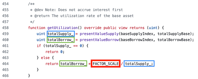
We don’t know at this point what scale totalSupply_ and totalBorrow_ (blue box and green box) are using, but it’s reasonable to assume they are using the same scale (number of decimals) and thus their scales will cancel out (return line 464). Since the numerator is multiplied by FACTOR_SCALE, (red box) the utilization percentage will be measured with 18 decimals.
Now let’s compare the current value of getUtilization() on Etherscan to what the Compound App shows

The current utilization of 904869679838357231 translates to 90.49% when divided by FACTOR_SCALE (and rounded to two decimals). It is indeed using 18 decimals.
The functions presentValueSupply and presentValueBorrow are not terms we expect the reader to be familiar with yet — but these can be thought of as the dollar value of the total capital available for lending and the total borrowed dollars respectively.
Step 3: Optimal utilization, or kink — are in the range [0-1e18]
In our article on Interest Rates in DeFi, we noted that popular interest rate models are piecewise functions with a notion of an “optimal” utilization. Compound V3 refers to this as the “kink” — when the interest rates start rising more sharply. These two different terms refer to the exact same concept.
At the time of writing, the optimal utilization for USDC on Ethereum is 93% as shown below.

Because utilization is measured with an 18 decimal fixed point number, the borrowKink and supplyKink are measured with 18 decimal fixed point numbers also. The interest rate function directly compares the two as we will see in an upcoming next section.
Step 4: mulFactor()
Programmers familiar with the mulDivDown from other fixed point libraries will have an easy time understanding this function.
It takes two fixed point numbers and multiplies them to produce another fixed point number. The function is shown below
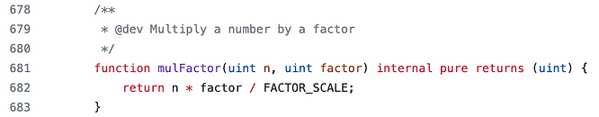
Since we are multiplying two numbers with 18 decimals together, we need to divide by FACTOR_SCALE to avoid having an 36-decimal output.
Just think of the function as “it multiplies two 18 decimals numbers together and returns an 18 decimal number representing their product.”
Step 5: getSupplyRate() returns decimal numbers on the factor scale
We are now ready to see that Compound V3 uses a 1e18 scale to measure interest rates.
Compound uses a piece-wise linear function as we discussed in our article on interest rates. Below is the getSupplyRate() function, which returns the current interest rate earned by lenders as determined by the current utilization rate. We know that mulFactor(...) returns FACTOR_SCALE (18 decimal) numbers. Therefore, we know that supplyPerSecondInterestRate (yellow circle) must also be a FACTOR_SCALE number or we would be adding numbers with a misaligned decimal. Therefore, the function getSupplyRate() returns FACTOR_SCALE decimals.

The function getBorrowRate behaves the same way, so we will not include that here.
The parameters of the curve — the intercepts, slopes, and kink — can all be adjusted by governance.
Calculating hypothetical interest rates
To calculate interest rates as a function of utilization, the user can get the current utilization using getUtilization() and plug that into getSupplyRate() and getBorrowRate().
contract GetCurrentRatesComet {
function getRates(IComet comet)
external
returns (uint64, uint64) {
uint64 private constant SECONDS_PER_YEAR = 365 * 24 * 60 * 60;
uint256 utilization = comet.getUtilization();
// these are 18 decimal fixed point numbers
// measuring interest per second
uint64 supplyRate = comet.getSupplyRate();
uint64 borrowRate = comet.getBorrowRate();
// return them as APR
return (supplyRate * SECONDS_PER_YEAR,
borrowRate * SECONDS_PER_YEAR);
}
}
Interest Rate Accrual
We have only shown how Compound calculates interest rates at a snapshot in time. In a later article we will show how it compounds and accrues interest.
Summary
The unit of time for interest rates are seconds. They are measured in 18 decimal precision. Utilization is also measured with 18 decimal precision.
Learn more with RareSkills
Please see our Blockchain Bootcamp to learn more.
Originally Published January 4, 2024