The P = NP problem asks: “If we can quickly verify a solution to a problem is correct, can we also quickly compute the solution?” Most researchers believe the answer is no, i.e., P ≠ NP.
By understanding the P vs NP problem, we can see how Zero Knowledge Proofs (ZKPs) fit into the larger field of computer science and comprehend what ZKPs can and cannot do.
It is far easier to “get” Zero Knowledge Proofs by relating them to the P vs NP problem.
This tutorial has three parts:
- Explaining the P vs NP problem
- Expressing problems and solutions as a Boolean formula
- P vs NP and how they relate to Zero Knowledge Proofs
Prerequisites
We assume the reader is familiar with time complexity and big notation.
We say an algorithm takes polynomial time if it runs in time or faster, where is the size of the input and is a non-negative constant. We may refer to algorithms that run in polynomial time or faster as efficient algorithms because their running time doesn’t grow too quickly with the input size.
We say an algorithm takes exponential time or is expensive if it runs in where is a constant greater than 1 and is the size of the input because the algorithm becomes exponentially slow as the size of the input increases.
Part 1: Explaining the P vs NP problem
Problems in P are problems that are both easy to solve and easy to verify solutions for.
Problems that can be solved in polynomial time and whose solutions can be verified in polynomial time are called problems in P.
Here are some example problems that are easy to compute and verify solutions for. These tasks might be performed by different parties, one doing the computation and another checking the results are valid:
P Example 1: Sorting a list
We can efficiently sort a list, and we can efficiently verify that a list is sorted.
-
Solving: Sorting the list takes time (for example, using mergesort), which is polynomial time. Although is not a polynomial, we know that and therefore , so our algorithm’s running time is bounded above by some polynomial, which is the requirement for “polynomial time.”
-
Verifying: We can verify the list is sorted by traversing the list and checking that each item is greater than its left neighbor, which would take time.
P Example 2: Returning the index of a number in a list, if it occurs in the list
We can efficiently search to see if a number is in a list and then even more efficiently verify that the number is present if we know the index it is in.
-
Solving: For example, given the list
[8, 2, 1, 6, 7, 3], we need time to determine if the number7is in the list. -
Verifying: But if we give you the list and say 7 is at index 4, you can verify the number is in the list at that position in time. Searching for an item, if we aren’t told its position, takes time in the general case since we have to search through the list. If we’re told the supposed location of the item, it takes time to verify that the item is, in fact, in the list at that location.
P Example 3: Determining if two nodes in a graph are connected
We can efficiently determine if two nodes in a graph are connected by using breadth-first search — start at a node, then visit all of its neighbors except nodes we’ve already visited, then search the neighbors of the neighbors, and so forth.
-
Solving: Discovering the path between nodes using breadth-first search will take time, where is the number of nodes in the graph and is the number of edges. The number of edges cannot exceed , so we can treat as in the worst case.
-
Verifying: We can verify the proposed path is valid in time simply by following the proposed path to see if the two points really are connected by that path.
In all the examples above, both computing and verifying the solution can be done in polynomial time.
The Witness
A witness in computer science is proof that you solved the problem correctly. In the examples above, the witness is the correct answer to the problem. For the examples above, these are things we could use as a witness:
- The sorted list
- The index where a number appears in the list
- The path between two nodes in a graph
We will see later that a witness does not necessarily have to be the solution to the original problem. It could also be a solution for an alternative representation of the same problem.
Problems in PSPACE: Not all problems have solutions that can be efficiently verified
Problems that require exponential resources to solve and verify are called problems in PSPACE. The reason they are called PSPACE is that although they might take exponential time to solve, they don’t necessarily require exponential memory space to run the search.
This class of problems has been researched extensively, yet no efficient algorithm to solve them has been discovered. Many researchers believe no efficient algorithm to solve these problems exists at all. If an efficient solution to these problems could be discovered, it would also be possible to reuse the algorithm to break all modern encryption and fundamentally alter computing as we know it.
Despite significant incentives for finding efficient solutions to these problems, evidence suggests such solutions likely do not exist. These problems are so challenging that you cannot provide easily verifiable proof (witness) even if you solve them correctly.
Examples of problems in PSPACE
PSPACE Example 1: Finding the optimal Chess move

Suppose we ask a powerful computer, “Given this chess board with the pieces in this position, what is the optimal next move?”
The computer responds with “move the black pawn on f4 to f3.”
How can you trust the computer is giving you the correct answer?
There is no efficient way to check—you must do the same work the computer did. This involves doing a full search through all possible future board states. There’s no witness the computer could provide us that would allow us to confirm that “move the black pawn on f4 to f3” is actually the next best move. In this way, the nature of this problem is very different from the examples in the previously discussed: we cannot efficiently verify that the claimed optimal move is the true optimal move.
In this example, the “witness” presented by the computer consists of all potential future game states. However, the massive volume of this data makes it practically impossible to verify the accuracy of the solution efficiently.
PSPACE Example 2: Determining if regexes (regular expressions) are equivalent
The two regexes, a+ and aa*, match the same strings. If a string matches the first regex, it will also match the second, and vice versa.
However, checking if two arbitrary regexes are equivalent takes exponential time to compute. Even if a powerful computer told you they match the same strings, there is no short proof (witness) the computer can give you to show the answers are correct. Similar to the chess example, you’d have to search a very large space of strings to check if the regexes are equivalent, and that will take exponential time.
Both Chess and Regex equivalence have a common characteristic in that they both require exponential resources to find answers and exponential resources to verify the answers.
Problems even more computationally intensive than PSPACE
There are problems that are so difficult that they require exponential time and exponential memory to solve, but those problems are usually theoretical and don’t frequently show up in the real world.
An example of such a problem is Checkers with a rule that pieces can never move into a position that recreates an earlier board state. In order to ensure we don’t repeat a board state for a game as we explore the space of possible moves, we have to keep track of all the board states that have already been visited. Since the length of the game can be exponential in the board size, the memory requirements are also exponential.
Problems in NP: Some problems can be quickly verified but not quickly computed
If we can quickly verify the solution to a problem, then the problem is in NP. However, finding the solution might require exponential resources.
Any problem whose proposed solution (witness) can be quickly verified as correct is an NP problem. If the problem also has an algorithm for finding the solution in polynomial time, then it is a P problem. All P problems are NP problems, but it is extremely unlikely that all NP problems are also P problems.
Examples of problems in NP. These are explained in more detail below:
- Computing the solution to a Sudoku puzzle — verifying the proposed solution to a Sudoku puzzle.
- Computing the 3-coloring of a map (if it exists) — verifying a proposed 3-coloring of a map.
- Finding an assignment to a Boolean formula that results in true — verifying the proposed assignment causes the formula to result in true.
Note: NP stands for non-deterministic polynomial. We won’t get into the jargon about where that name came from; we’re just giving the name so the reader doesn’t mistakenly think it stands for “not polynomial time.”
Examples of problems in NP
NP Example 1: Sudoku
In the game Sudoku, a player is given a grid with some numbers filled in. The goal is for the player to fill in the rest of the grid with numbers 1-9 such that no number occurs more than once in any row, column, or box (the ones outlined by bold lines). The following images from Wikipedia illustrate this. In the first image, we see the 9x9 grid as given to the player. In the second image, we see the player’s solution.


Given a Sudoku puzzle solution, we can quickly verify the solution is correct simply by looping over the columns, rows, and subgrids. The witness can be verified in polynomial time.
However, computing the solution requires significantly more resources — there are an exponential number of combinations to search. For a grid, this is not difficult for a computer. However, if we allow the Sudoku puzzle to be arbitrarily large: each side has size , where is a multiple of 9. In that case, the difficulty of finding the solution grows exponentially with .
NP Example 2: Three-coloring a map
Any 2D map of territories can be “colored” with just four colors (see the four color theorem). That is, we can assign a unique color (one of four colors) to each territory such that no neighboring territories share the same color. For example, the following image (from Wikipedia) shows the United States colored with four colors: pink, green, yellow, and red. Take a moment to look at the verify that no two touching states have been given the same color:

The three-coloring problem asks whether a map can be colored using just three colors instead of four. Discovering a three-coloring (if it exists) is a computationally intensive search problem. However, verifying a proposed 3-coloring is easy: loop through each of the regions and check that no neighboring regions have the same color of the territory currently being checked.
It turns out that it is not possible to 3-color the United States.
The reasons a particular map cannot be 3 colored vary, but in the case of the United States, Nevada (the red region in the map below) is surrounded by five territories. We color Nevada with one color, then we must alternate the colors of its neighboring territories. However, when we finish circling the neighbors of Nevada, we will end up with a territory having neighbors with three colors on its boundaries, leaving no valid color for the uncolored territory.

Here is a quick and interesting video about 3-coloring maps if you want to learn more about this problem.
However, it is possible to 3-color Australia:

Not all maps can be three-colored. Computing a three-coloring for an arbitrary 2D map, if it exists, cannot be done efficiently — it typically requires a brute-force search that may take exponential time.
However, if someone solves a three-coloring, it is easy to verify their solution.
The relationship between P, NP, and PSPACE
Computational resources for each class
The table below summarizes the computational resources required for each class of problem:
| Category | Compute Time | Verification Time |
|---|---|---|
| P | Must be polynomial or better | Must be polynomial or better |
| NP | No Requirement | Must be polynomial or better |
| PSPACE | No Requirement | No Requirement |
Hierarchy of Difficulty between P, NP, and PSPACE
Any problem that requires exponential resources to verify the witness for is a PSPACE (or harder problem). If one has exponential resources to verify witnesses for PSPACE problems, that person can trivially compute solutions for any P or NP problem. Therefore, all P and NP problems are a subset of PSPACE problems, as illustrated in the figure below.
In other words, if you have a powerful enough computer to solve or verify a class of problem in the larger circle, you can solve or verify a subset of it:

The P vs NP problem
P is the class of problems that can be solved and verified efficiently, while NP is the class of problems that can be verified efficiently. The “P vs NP” question asks, simply, whether these two classes are the same.
If P = NP, it would mean that whenever we can find an efficient method for verifying a solution, we can also find an efficient method for finding that solution. Remember that finding a solution is always at least as hard as verifying it. (By definition, solving a problem includes finding the correct answer, which means an algorithm that solves the problem is also verifying its answer in the process).
If P = NP is true, that means there is an efficient algorithm for computing Sudoku puzzles (of arbitrary size) and finding if a three coloring exists. It also means there is an efficient algorithm to break most modern cryptographic algorithms.
Currently, it remains unproven whether P and NP are the same set. Although numerous attempts have been made to find efficient algorithms for NP problems, all evidence suggests that such algorithms do not exist.
Similarly, whether efficient solutions or verification mechanisms exist for PSPACE problems remains open. While researchers widely speculate that P ≠ NP and NP ≠ PSPACE, no formal mathematical proof exists for these conclusions. Therefore, despite extensive efforts, efficient solutions for NP problems and efficient verification methods for PSPACE problems remain undiscovered.
For practical purposes, we can assume P ≠ NP and NP ≠ PSPACE. In fact, we implicitly make that assumption when we trust important data to modern cryptography algorithms.
Part 2: Expressing problems and solutions as Boolean formulas
What ties P and NP problems together is that their solution can be quickly verified. It would be extremely useful if we could describe all those (P and NP) problems and their solutions in a common language. That is, we want an encoding of the problem that works for problems as diverse as proving a list is sorted, to proving a Sudoku puzzle is solved, to proving we have a three coloring.
Verifying a solution to a problem in NP or P can be accomplished by verifying a solution to a Boolean formula that models the problem.
What we mean by “a Boolean formula that models the problem” will become clear as we describe what we mean by “a solution to a Boolean formula” and looking at some example modeling problems with Boolean formulas.
Solutions to a Boolean formula
To express a Boolean formula, we use the operator to be the Boolean NOT, to be the Boolean AND, and to be the Boolean OR. For example, evaluates to true if and only if and are both true. evaluates to true if and only if is true and is false.
Suppose we have a bunch of Boolean variables , , , and a Boolean formula:
The question is: can we find values for such that is true? For the above formula, we can. Writing for true and for false, we can write our solution as:
Plugging the solution into the formula yields:
That was easy to verify, but discovering the solution for a very large Boolean formula could require exponential time. Finding a solution to a Boolean formula is an NP problem itself — it may require exponential resources to find the solution, but verifying it can be done in polynomial time.
But we must emphasize: our use of Boolean formulas is not to solve them — only to verify proposed solutions for them.
All problems in P and NP can be verified by transforming them into boolean formulas and showing a solution to the formula
In the following examples, the input is a P or NP problem and the output is a Boolean formula. If we know the solution to the original problem, then we will also know the solution to the Boolean formula.
Our intent is to show we know the witness for the original problem — but in Boolean form.
Example 1: checking if a list is sorted using a Boolean formula
Consider one-bit binary numbers and . The following truth table returns true when :
| A | B | A > B |
|---|---|---|
| 0 | 0 | 0 |
| 0 | 1 | 0 |
| 1 | 0 | 1 |
| 1 | 1 | 0 |
The column can be modeled with the expression , which returns true in the only row where is one.
Now consider a table that expresses :
| A | B | A = B |
|---|---|---|
| 0 | 0 | 1 |
| 0 | 1 | 0 |
| 1 | 0 | 0 |
| 1 | 1 | 1 |
The column can be modeled with the expression . returns true when and and returns true when and are both zero.
The expressions for one bit numbers:
will come in handy shortly.
Now how do we compare binary numbers of more than one bit?
Binary comparison by most significant different bit
Suppose you start from both numbers’ leftmost Most Significant Bit (MSB) and move towards the right Least Significant Bit (LSB). At the first bit, where the two numbers differ:
If has a value of at that bit and has a value of , then .
The following animation illustrates the algorithm detecting that :

If , then all of the bits are equal. means is also true:

If P < Q, then we will detect that on the first bit where Q is 1 and P is 0:

Suppose, without loss of generality, that we number the bits in as and the bits in as .
If then one of the following must be true:
- and
- and and
- and and and
We can combine the bullet points into a single equation.
Recall our Boolean expressions that modeled one bit equality and comparison:
We can substitute the expressions for and formula in to the equation above. To avoid a wall of math, we show the operations in video form below:
The final Boolean formula that expresses , for 4 bits, is:
Let’s call a Boolean expression that compares two binary numbers in the manner described above a
“comparison expression.”
Checking if a list is sorted
Given a Boolean formula to compare numbers of a fixed size, we can repeatedly apply the comparison expression to each pair of adjacent elements in the list and combine the comparison expressions using the AND operation. The list is sorted if and only if the AND of all the comparison expressions is true.
Thus, we see that a witness that proves a list is sorted does not have to be the sorted list. It can also be the input to Boolean formula that we created above that results in the formula returning true.
Example 2: A 3-coloring as a Boolean formula
Let’s look at our map of Australia again:
To model the solution as a Boolean formula, the formula needs to encode the following facts:
- Each territory has one of three colors
- Each territory has a different color from its neighbor
For example, to say Western Australia is either green, blue, or red, we need to create three variables WESTERN_AUSTRALIA_GREEN, WESTERN_AUSTRALIA_BLUE,WESTERN_AUSTRALIA_RED. To avoid long variable names, let’s call it WA_G, WA_B, and WA_R. Our Boolean formula is then:
(WA_G ∧ ¬WA_B ∧ ¬WA_R) ∨ (¬WA_G ∧ WA_B ∧ ¬WA_R) ∨ (¬WA_G ∧ ¬WA_B ∧ WA_R)
In other words:
"(West Australia is green AND West Australia is NOT blue AND West Australia is NOT red)
OR
(West Australia is NOT green AND West Australia is blue AND West Australia is NOT red)
OR
(West Australia is NOT green AND West Australia is NOT blue AND West Australia is red)"
Coloring the Boolean formula for emphasis:
(WA_G ∧ ¬WA_B ∧ ¬WA_R) ∨ (¬WA_G ∧ WA_B ∧ ¬WA_R) ∨ (¬WA_G ∧ ¬WA_B ∧ WA_R)
Let’s call the formula above the color assignment constraint.
We use Boolean variables to encode the assigned color of a territory. Since a Boolean variable can only hold two values, but a territory can be one of three colors, each territory is assigned three Boolean variables, one for each color. If a territory is assigned a particular color, the corresponding variable is set to true and the others are set to false.
The above formula is true if and only if the territory of Western Australia is assigned exactly one color.
Neighboring color constraint
Next, we want to write a formula which expresses that WA has a different color than it’s neighbor. We make three variables for SA (South Australia) like we did for WA. Now, our formula simply says, “for each color, WA and SA are not both that color”. This is equivalent to saying “WA and SA are not the same color.” Let’s use the variable names SA_G, SA_B, and SA_R to refer to the color assignment of South Australia (which neighbors Western Australia). We use the formula below to express that they have different colors:
¬(WA_G ∧ SA_G) ∧ ¬(WA_B ∧ SA_B) ∧ ¬(WA_R ∧ SA_R)
In other words:
it is NOT the case that (West Australia is green AND South Australia is green)
AND
it is NOT the case that (West Australia is blue AND South Australia is blue)
AND
it is NOT the case that (West Australia is red AND South Australia is red)"
The above formula will be satisfied if and only if Western Australia and South Australia were not assigned the same color. Let’s call the formula above the boundary constraint.
We need to apply the color assignment constraint to each territory and the different color constraint to each pair of neighbors, then AND all the constraints together.
A formula to model a 3-coloring of Australia
We now show the final Boolean formula that verifies a valid 3 coloring for Australia. Here are the territories labelled:
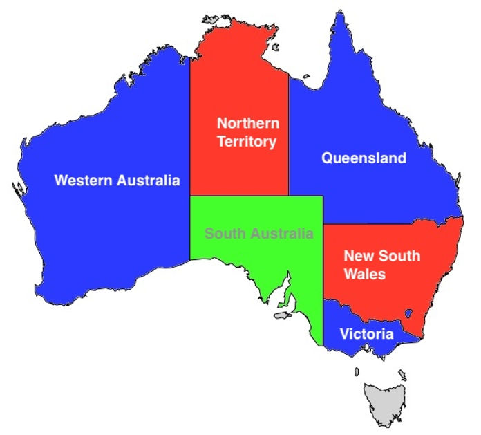
First, we assign each territory a variable name:
WA= West AustraliaSA= South AustraliaNT= Northern TerritoryQ= QueenslandNSW= New South WalesV= Victoria
Color constraints: Each of the six territories has exactly one color:
-
(WA_G ∧ ¬WA_B ∧ ¬WA_R) ∨ (¬WA_G ∧ WA_B ∧ ¬WA_R) ∨ (¬WA_G ∧ ¬WA_B ∧ WA_R)
-
(SA_G ∧ ¬SA_B ∧ ¬SA_R) ∨ (¬SA_G ∧ SA_B ∧ ¬SA_R) ∨ (¬SA_G ∧ ¬SA_B ∧ SA_R)
-
(NT_G ∧ ¬NT_B ∧ ¬NT_R) ∨ (¬NT_G ∧ NT_B ∧ ¬NT_R) ∨ (¬NT_G ∧ ¬NT_B ∧ NT_R)
-
(Q_G ∧ ¬Q_B ∧ ¬Q_R) ∨ (¬Q_G ∧ Q_B ∧ ¬Q_R) ∨ (¬Q_G ∧ ¬Q_B ∧ Q_R)
-
(NSW_G ∧ ¬NSW_B ∧ ¬NSW_R) ∨ (¬NSW_G ∧ NSW_B ∧ ¬NSW_R) ∨ (¬NSW_G ∧ ¬NSW_B ∧ NSW_R)
-
(V_G ∧ ¬V_B ∧ ¬V_R) ∨ (¬V_G ∧ V_B ∧ ¬V_R) ∨ (¬V_G ∧ ¬V_B ∧ V_R)
Boundary constraints: Each neighboring territory does not share a color
Next, we iterate through the boundaries and compute a boundary constraint for those neighbors. The video below shows the algorithm in action. We show the final set of formulas for the boundary conditions after the video:
- Western Australia and South Australia:
¬(WA_G ∧ SA_G) ∧ ¬(WA_B ∧ SA_B) ∧ ¬(WA_R ∧ SA_R)
- Western Australia and Northern Territory:
¬(WA_G ∧ NT_G) ∧ ¬(WA_B ∧ NT_B) ∧ ¬(WA_R ∧ NT_R)
- Northern Territory and South Australia:
¬(NT_G ∧ SA_G) ∧ ¬(NT_B ∧ SA_B) ∧ ¬(NT_R ∧ SA_R)
- Northern Territory and Queensland:
¬(NT_G ∧ Q_G) ∧ ¬(NT_B ∧ Q_B) ∧ ¬(NT_R ∧ Q_R)
- South Australia and Queensland:
¬(SA_G ∧ Q_G) ∧ ¬(SA_B ∧ Q_B) ∧ ¬(SA_R ∧ Q_R)
- South Australia and New South Wales:
¬(SA_G ∧ NSW_G) ∧ ¬(SA_B ∧ NSW_B) ∧ ¬(SA_R ∧ NSW_R)
- South Australia and Victoria:
¬(SA_G ∧ V_G) ∧ ¬(SA_B ∧ V_B) ∧ ¬(SA_R ∧ V_R)
- Queensland and New South Wales:
¬(Q_G ∧ NSW_G) ∧ ¬(Q_B ∧ NSW_B) ∧ ¬(Q_R ∧ NSW_R)
- New South Wales and Victoria:
¬(NSW_G ∧ V_G) ∧ ¬(NSW_B ∧ V_B) ∧ ¬(NSW_R ∧ V_R)
We create a Boolean formula by taking the Boolean AND of the 15 formulas mentioned above… Having an assignment to the variables that results in the result of the Boolean expression being true is equivalent to having a valid 3-coloring of Australia.
In other words, if we know a valid 3-coloring for Australia, then we also know an assignment to the Boolean formula constructed above.
The Boolean Formula must be constructable in polynomial time
We only need to take a polynomial number of steps to construct this Boolean formula for 3-coloring. Specifically, we need:
- 3 color constraints per territory
- At most N neighboring color constraints per territory
It is a requirement that the steps taken to construct the Boolean formula be done in polynomial time. If it takes an exponential number of steps, then the Boolean formula will be exponentially large, and the witness will be exponentially large — and not verifiable in polynomial time.
Summary of using Boolean expressions to model problems and proposed solutions
All problems in P and NP can be expressed as a Boolean formula that outputs true if we know the corresponding variable assignment (witness), which encodes a correct solution to the original problem.
Now that we have a standard language for efficiently demonstrating a solution to a problem, we are one step closer to a standard method for demonstrating that we have a solution to a problem — without revealing the solution, i.e., Zero Knowledge Proofs.
Part 3: P vs NP and ZK Proofs
How P = NP relates to ZK Proofs
The “knowledge” in Zero Knowledge Proofs refers to knowledge of the witness.
ZK proofs are concerned with the verification aspect of computation. That is, given that you have found a Sudoku solution or a 3-coloring of a map, can you give someone evidence (witness) that would allow them to efficiently verify that your solution is correct?
ZK proofs seek to demonstrate that you know the witness without revealing it.
ZKPs only work with P or NP problems. They are not usable for problems which we can’t verify efficiently.
If we don’t have a mechanism to efficiently prove regexes are equivalent, or that a certain move in chess is optimal, then ZK proofs cannot magically enable us to produce such an efficient proof.
For both P and NP problems, the verification of the solution can be done efficiently. ZK enables verifying the solution is valid while concealing the details of the computation. Furthermore, ZK cannot help you discover a solution to a Sudoku puzzle or discover a 3-coloring of a map. However, it can help you prove to another party that you have a solution, if you already computed it.
The connection between P vs NP and Zero Knowledge Proofs
All problems with solutions that can be quickly verified can be converted into a Boolean formula.
Being able to convert any problem into a Boolean formula is not a cheat code for finding the answer efficiently. Solving an arbitrary Boolean expression is an NP problem, and finding a solution to it may be difficult.
The size of the Boolean formula is important. Going back to our chess example, if you try to model every state with a Boolean formula, then the size of your formula will be exponentially large. Therefore, the only feasible problems are NP or P, which have reasonably sized Boolean formulas that model them.
In the ZK literature, we often refer to Boolean formulas as Boolean circuits.
Creating a zero knowledge proof for a problem boils down to translating the problem to a circuit, as demonstrated when proving a three-coloring for Australia or validating a sorted list. Then, you prove you have valid input to the circuit (the witness), which ultimately transforms into zero knowledge proof.
The ability to efficiently verify a solution to a problem is a prerequisite for creating a zero knowledge proof that you have a solution. One must be able to construct a Boolean circuit to model the solution efficiently. However, for problems like determining optimal Chess moves, which belong to PSPACE, this approach results in exponentially large circuits, making them impractical.
In conclusion, zero knowledge proofs are feasible only for problems within P and NP, where efficient solution verification is possible. Without efficient verification, creating a zero knowledge proof for a problem becomes infeasible.
Learn more
Please see the RareSkills ZK Book for more topics in zero knowledge proofs.
Technicalities
Some concepts have been simplified in this article to make them as understandable as possible to someone seeing them for the first time. The information presented here is sufficient to explain what ZK proofs can and cannot do. For those interested in pursuing the subject further, here are some clarifications:
-
A chess board of a fixed size cannot be assigned a difficulty level because the difficulty of the problem cannot be expressed as . Technically, we say chess of an arbitrary size is PSPACE. It might be confusing to think of a chess board, but one can simply specify that the extra spaces don’t have any pieces in them at the starting position.
-
Chess has a lesser known rule that if no capture move has taken place and no pawn has moved for the last 50 moves, then a player can call a draw. This places a bound on the search space that puts it in PSPACE. If this rule is removed, then this version of chess is in EXPSPACE — a category of problems that requires exponential time and exponential memory size to compute.
-
Some NP problems can be solved in sub exponential time, but for practical purposes, they take exponential time to solve. For example is technically sub-exponential, but it is still exponentially difficult.
-
Very powerful heuristics for finding solutions to some NP problems exist. Although three coloring takes exponential time to solve, many instances of the problem of reasonable size can be solved quickly. For example, here are benchmark problems of maps with 200 territories and valid 3 colorings. Clever algorithms are able to find the solution without exploring an exponentially large search space. However, for any heuristics designed to speed up solving an NP problem, it is possible to create a pathological instance of problem that is designed to exploit the heuristic and make it worthless. Nevertheless, the heuristics work well for the typical instance of a realistic example of the problem.
Originally Published April 10, 2024